SOLVING THE STEADY AND UNSTEADY 2D HEAT CONDUCTION EQUATION BY USING ITERATIVE SOLVERS IN MATLAB

AIM :

To solve steady and unsteady 2D heat conduction equation by using the point Iterative Techniques such as jacobi, Gauss siedel and SOR(Succesive Over Relaxation) using Matlab

Initial temperature :

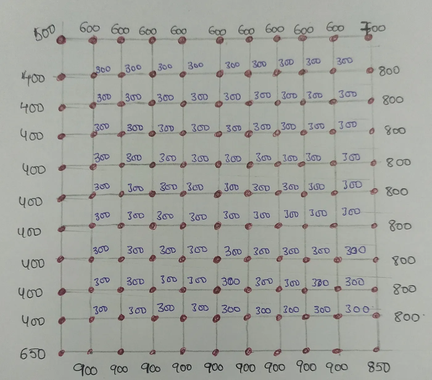
Problem statement:

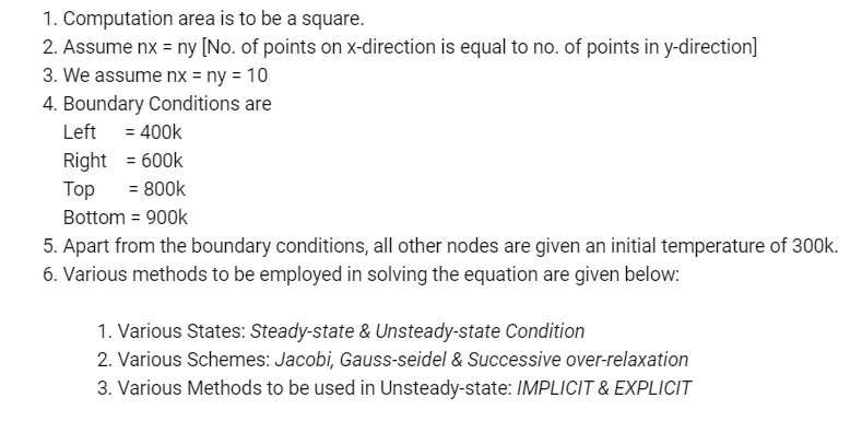
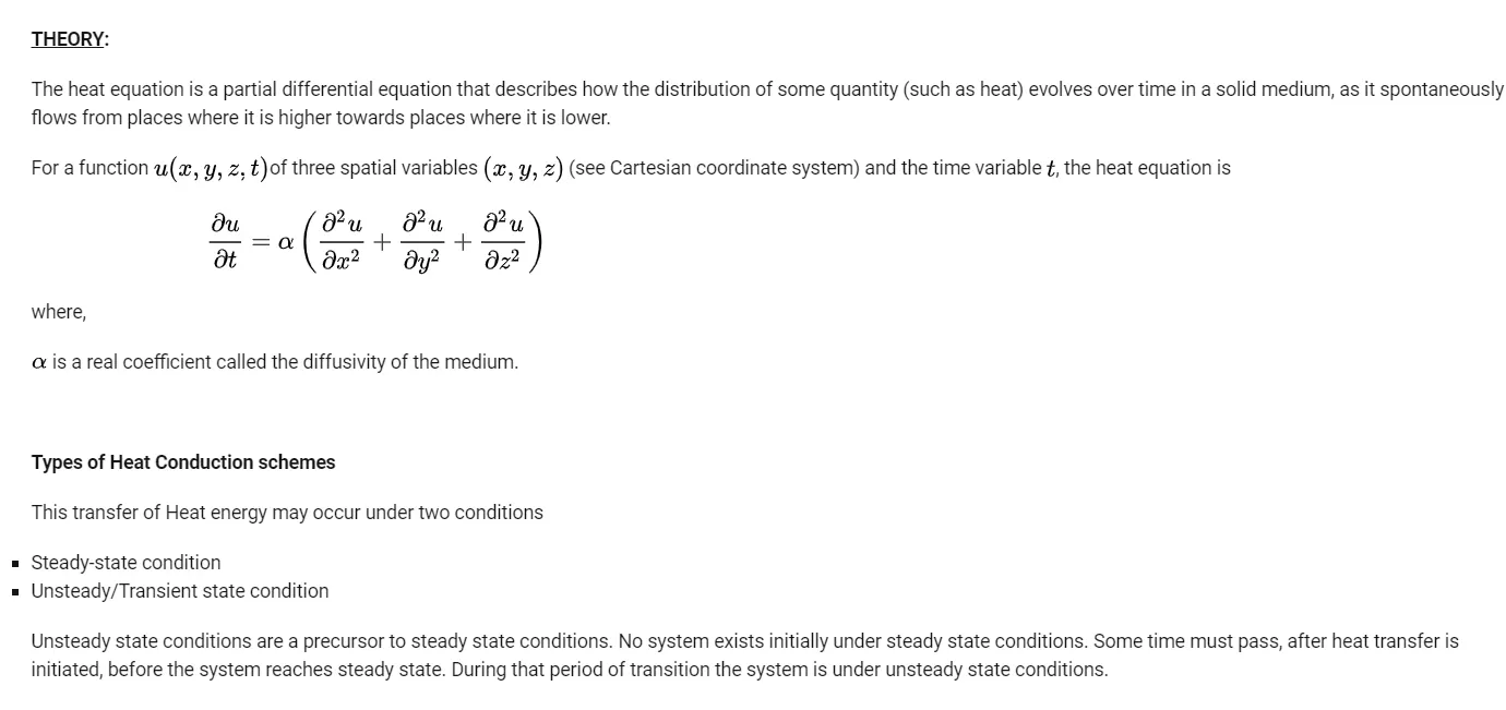
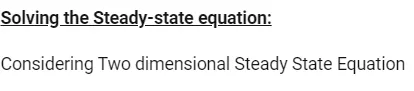
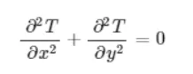
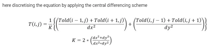
Steady state Matlab code :

%Solving the steady state equation by using different iterative solvers
clear all
close all
clc
%defining the inputs
nx=10;
ny=nx;
x=linspace(0,1,nx);
y=linspace(0,1,ny);
dx=x(2)-x(1);
dy=y(2)-y(1);
[xx,yy]=meshgrid(x,y);
%Defining the boundary conditions
T=300*ones(nx,ny);
T(1,:)=600;
T(end,:)=900;
T(:,1)=400;
T(:,end)=800;
%Rounding off the corner values
T(1,1)=(400+600)/2;
T(1,ny)=(600+800)/2;
T(nx,1)=(400+900)/2;
T(nx,ny)=(900+800)/2;
%creating a copy of T
Told=T;
%Tolerance error value and initializing the error value to a random number greater than 1
 tol=1e-4;
 error=500;
 k=(2*(dx^2+dy^2))/(dx^2*dx^2);
 %defining the iterative solvers
 iterative_solver=input('Enter the solver number either 1(jacobi) or 2(Gauss sidel) or 3(SOR) :  ');
 if iterative_solver==1
     tic;
     Tjacobi=jacobi_iter_steady(error,tol,xx,yy,nx,ny,dx,dy,T,k,Told)
     Time_in_jacobi_sec=toc
 elseif iterative_solver==2
         tic;
         Tgs=gs_iter_steady(error,tol,xx,yy,nx,ny,dx,dy,T,k,Told)
         Time_in_gs_sec=toc
 elseif iterative_solver==3
     tic;
     T_sor= SOR_iter_steady(error,tol,xx,yy,nx,ny,dx,dy,T,k,Told)
     Time_in_SOR_sec=toc
 end

Code Explanation:

1) At first Number of nodes have to be selected, Here the selected number of nodes =10x10=100

2) Value of dx and dy is calculated and boundary conditions are assigned.

3) Corner values of temperature are rounded off by taking the average.

4) Tolerance for steady state convergence is assumed which is equal to 1e-4 and at first error is to be assigned with a random value greater than 1 , here it is taken as 500.

5) According to the number which is inputed in the iterative solver that corresponding iteration technique is peformed by calling their respective function blocks.

6) Time for execution of each Iteration technique is calculated.

jacobi function code :

function T=jacobi_iter_steady(error,tol,xx,yy,nx,ny,dx,dy,T,k,Told)
jacobi_iter=1;
while(error>tol)
    for i=2:nx-1
        for j=2:ny-1
            term1=(Told(i-1,j)+Told(i+1,j))/(k*dx^2);
            term2=(Told(i,j-1)+Told(i,j+1))/(k*dy^2);
            T(i,j)=term1+term2;
        end
    end
    error=max(max(abs(Told-T)));
    Told=T;
    jacobi_iter=jacobi_iter+1;
    figure(1)
    [c,d]=contourf(xx,yy,T);
    colormap(jet)
    colorbar
    set(gca,'ydir','reverse')
    title_text=sprintf('Jacobi Iteration number = %d  for steady state',jacobi_iter);
    title(title_text)
    xlabel('xaxis')
    ylabel('yaxis')
    clabel(c,d)
    pause(0.03)
    
end
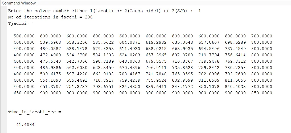
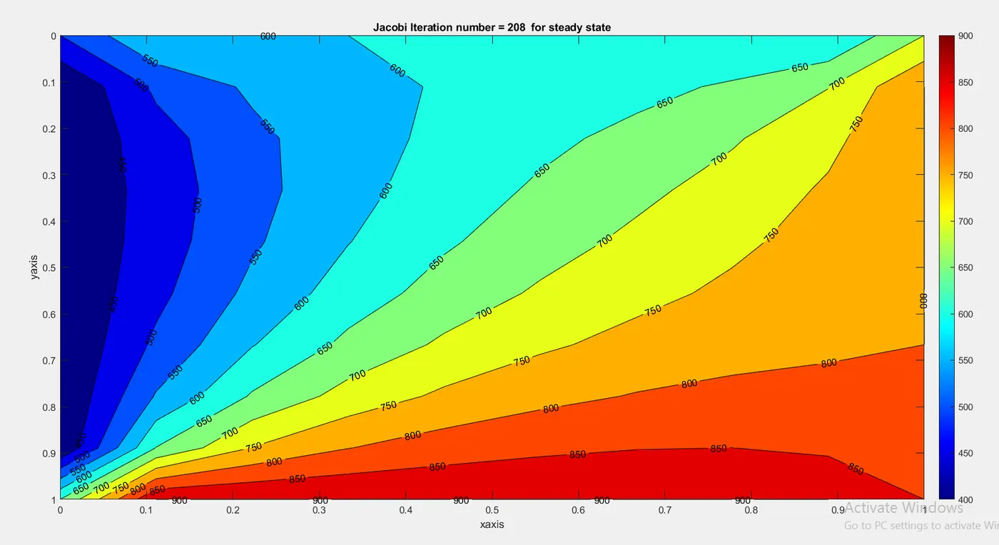
fprintf('No of iterations in jacobi = %d',jacobi_iter);
end

Code explanation :

1) At first the inner nodes are taken any random value here all inner nodes are taken at a temperature of 300K

2) The Iteration technique is performed until the the solution converges to the specified tolerance value.

3) While loop is the convergence loop it keep on executing until the error value is less than tolerance value

4)The temperature values have to be updated after each iteration otherwise the while loop will never stop.

5) In jacobi technique old values are used for all the nodes even though updated values are available

6) The temperature contour is plotted and we can observe how the solution converges for each and every iteration value

7) reverse the y axis value as the contour profile converges at point 1

Gauss siedel function code:

function T=gs_iter_steady(error,tol,xx,yy,nx,ny,dx,dy,T,k,Told)
gs_iter=1;
while(error>tol)
    for i=2:nx-1
        for j=2:ny-1
            term1=(T(i-1,j)+Told(i+1,j))/(k*dx^2);
            term2=(T(i,j-1)+Told(i,j+1))/(k*dy^2);
            T(i,j)=term1+term2;
        end
    end
    error=max(max(abs(Told-T)));
    Told=T;
    gs_iter=gs_iter+1;
    figure(2)
    [c,d]=contourf(xx,yy,T);
    colormap(jet)
    colorbar
    set(gca,'ydir','reverse')
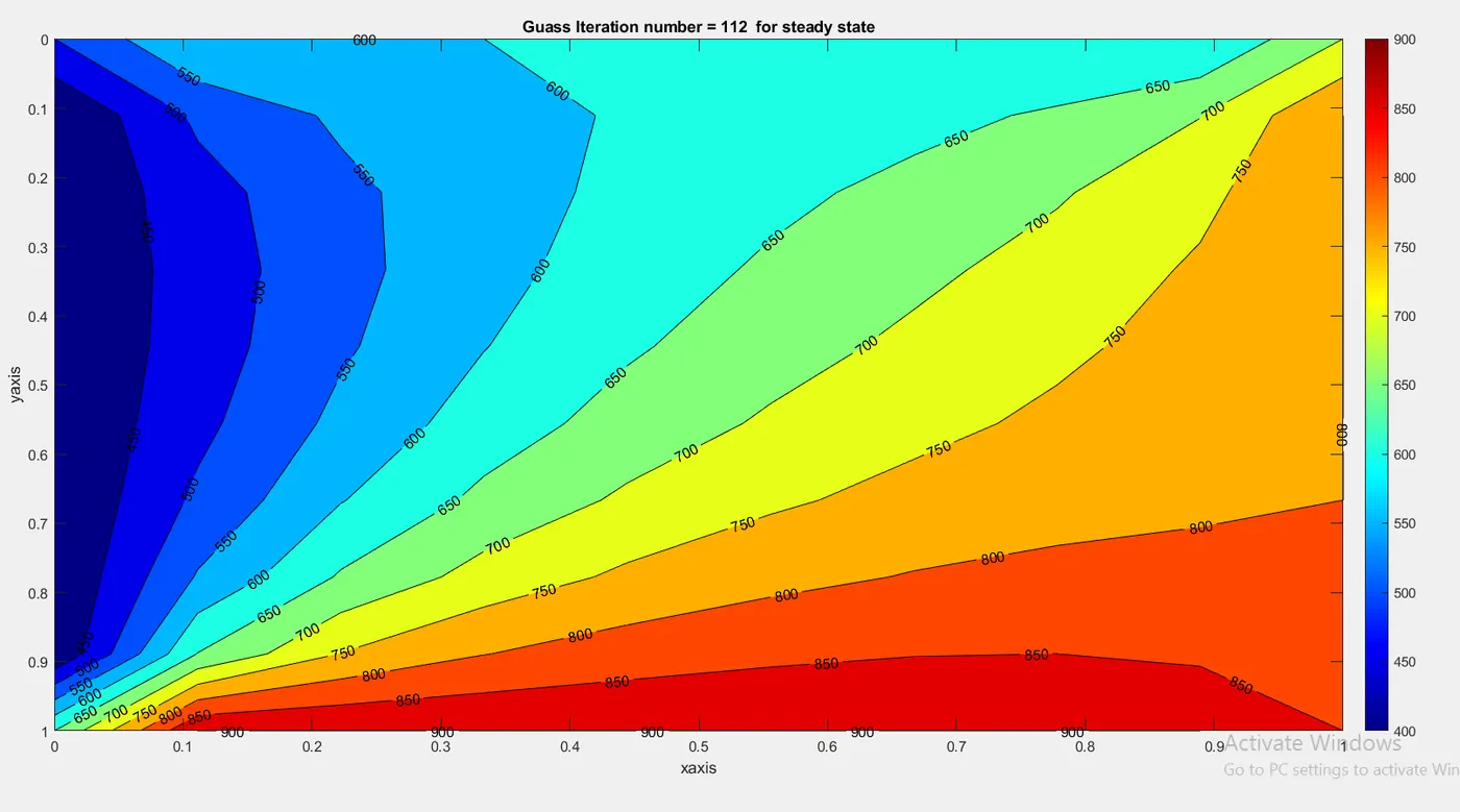
    title_text=sprintf('Guass Iteration number = %d  for steady state',gs_iter);
    title(title_text)
    xlabel('xaxis')
    ylabel('yaxis')
    clabel(c,d)
    pause(0.03)
end
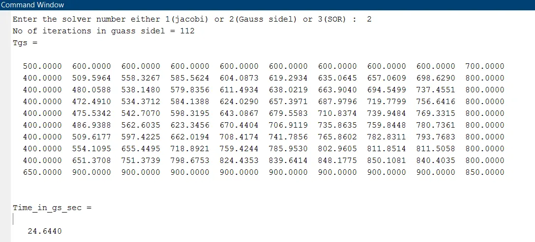
fprintf('No of iterations in guass sidel = %d',gs_iter);
end

Code explanation :

1) At first the inner nodes are taken any random value here all inner nodes are taken at a temperature of 300K

2) The Iteration technique is performed until the the solution converges to the specified tolerance value.

3) While loop is the convergence loop it keep on executing until the error value is less than tolerance value

4)The temperature values have to be updated after each iteration otherwise the while loop will never stop.

5) In Guass siedel technique updated values are used for all the nodes and for the nodes upadated value is not available old data is used

6) The temperature contour is plotted and we can observe how the solution converges for each and every iteration value

7) reverse the y axis value as the contour profile converges at point 1

SOR function code:

function T=SOR_iter_steady(error,tol,xx,yy,nx,ny,dx,dy,T,k,Told)
SOR_iter=1;
alpha=1.5;
while(error>tol)
    for i=2:nx-1
        for j=2:ny-1
            term1=(T(i-1,j)+Told(i+1,j))/(k*dx^2);
            term2=(T(i,j-1)+Told(i,j+1))/(k*dy^2);
            T_gs(i,j)=term1+term2;
            T(i,j)=(alpha*T_gs(i,j)+((1-alpha)*Told(i,j)));
        end
    end
    error=max(max(abs(Told-T)));
    Told=T;
    SOR_iter=SOR_iter+1;
    figure(3)
    [c,d]=contourf(xx,yy,T);
    colormap(jet)
    colorbar
    set(gca,'ydir','reverse')
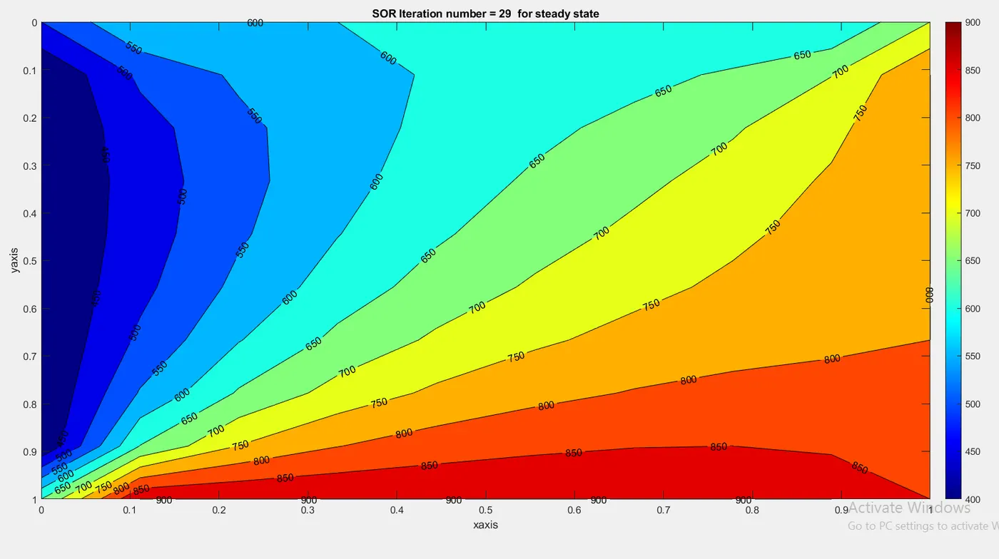
    title_text=sprintf('SOR Iteration number = %d  for steady state',SOR_iter);
    title(title_text)
    xlabel('xaxis')
    ylabel('yaxis')
    clabel(c,d)
    pause(0.03)
end
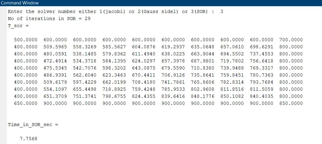
fprintf('No of iterations in SOR = %d',SOR_iter);
end

Code explanation :

1) At first the inner nodes are taken any random value here all inner nodes are taken at a temperature of 300K

2) The Iteration technique is performed until the the solution converges to the specified tolerance value.

3) While loop is the convergence loop it keep on executing until the error value is less than tolerance value

4)The temperature values have to be updated after each iteration otherwise the while loop will never stop.

5) In SOR technique a relaxation factor omega is used for scaling the guass siedel or jacobi technique and if omega varies from 0 to 1 Temperature iteration varies from no update to Jacobian or gauss siedel

6) The temperature contour is plotted and we can observe how the solution converges for each and every iteration value

7) reverse the y axis value as the contour profile converges at point 1

Comparision of the Techniques for steady state condition :

From the above 3 techniques SOR takes less time and few iterations to converge to the tolernce value if a desired omega value is choosen . If omega is too large the solution overshoots and takes more amount of time than jacobian and guass siedel at the same time it should not be too less.

Transient state Explicit method

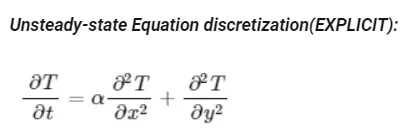
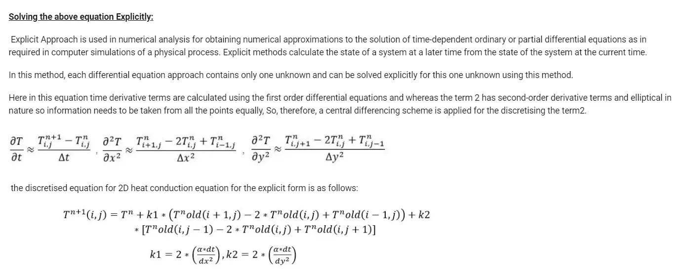
Explicit Transient state matlab code :

%solving 2D Transient heat conduction equation explicitly
clear all
close all
clc
%defining the inputs 
nx=10;
ny=nx;
x=linspace(0,1,nx);
y=linspace(0,1,ny);
dx=x(2)-x(1);
dy=y(2)-y(1);
dt=0.1;
%Thermal diffusivity 
diffusivity=0.014;
[xx,yy]=meshgrid(x,y);
%Defining the boundary conditions
T=300*ones(nx,ny);
T(1,:)=600;
T(end,:)=900;
T(:,1)=400;
T(:,end)=800;
%Rounding off the corner values
T(1,1)=(400+600)/2;
T(1,ny)=(600+800)/2;
T(nx,1)=(400+900)/2;
T(nx,ny)=(900+800)/2;
%creating a copy of T
Told=T;
%Tolerance error value and initializing the error value to a random number greater than 1
 tol=1e-4;
 error=500;
 k1=diffusivity*(dt/dx^2);
 k2=diffusivity*(dt/dy^2);
 CFL=k1+k2
 %defining the iterative solvers
 iterative_solver=1;
 if iterative_solver==1
     tic;
     [T,Convergence_error]=Transient_explicit(error,tol,xx,yy,nx,ny,T,k1,k2)
     Time_in_sec=toc
 end

Code explanation :

1) In Explicit method no iterative solvers are required because in the equation all are known values and the next time value can be directly calculated by substituting previous time step value

2) For explicit stability CFL < 0.5

Function code :

function [T,error]=Transient_explicit(error,tol,xx,yy,nx,ny,T,k1,k2)
Timesteps=1;
%At t=0sec
Told=T;

    for q=1:1220 %Time loop for acheiving the steady state solution
        %Space loop for calculation of Temperature at inner nodes except at boundary values for specific time step
    for i=2:nx-1
        for j=2:ny-1
            term1=Told(i,j);
            term2=k1*(Told(i+1,j)-2*Told(i,j)+Told(i-1,j));
            term3=k2*(Told(i,j+1)-2*Told(i,j)+Told(i,j-1));
            T(i,j)=term1+term2+term3;
        end
    end  
    %Error for steady state convergence
    error=max(max(abs(Told-T)));
    %Updating the  Temperture values for the calculation of next time steps i.e 0.1,0.2,...........122 sec
    Told=T;
    Timesteps=Timesteps+1;
figure(1)
    [c,d]=contourf(xx,yy,T);
    colormap(jet)
    colorbar
    set(gca,'ydir','reverse')
    title_text=sprintf('No of timesteps  = %d  for convergence to steadystate',Timesteps);
    title(title_text)
    xlabel('xaxis')
    ylabel('yaxis')
    clabel(c,d)
    end
end

Code explanation :

1) The first for loop is time loop and the second for loops are spacial loops

2)The time loop is executed for 1220 times so that the solution reaches to a steady state value

3) No linear equatiuons are solved so no ierative solver are used.

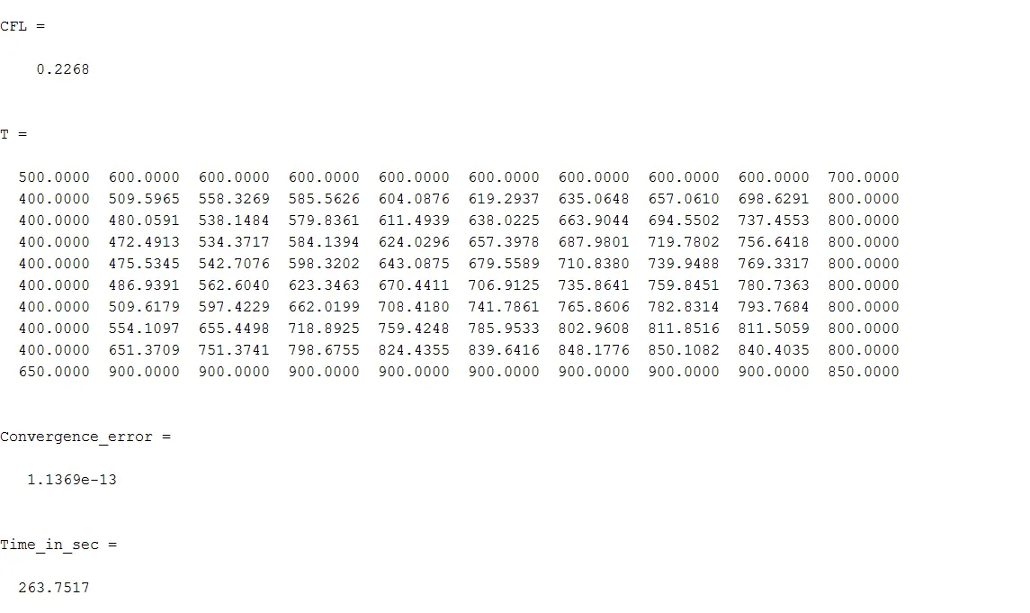
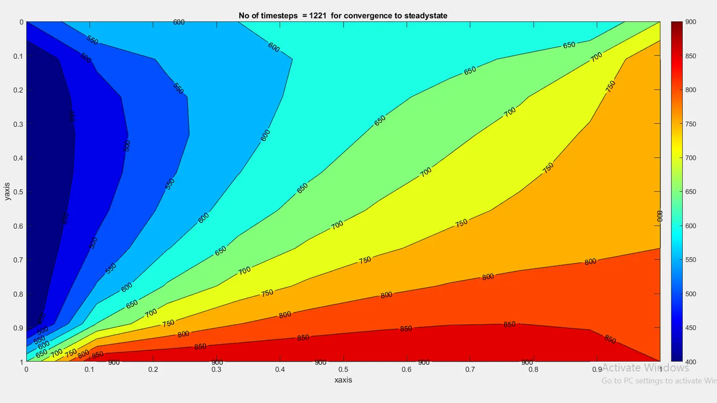
Transient state Implicit method

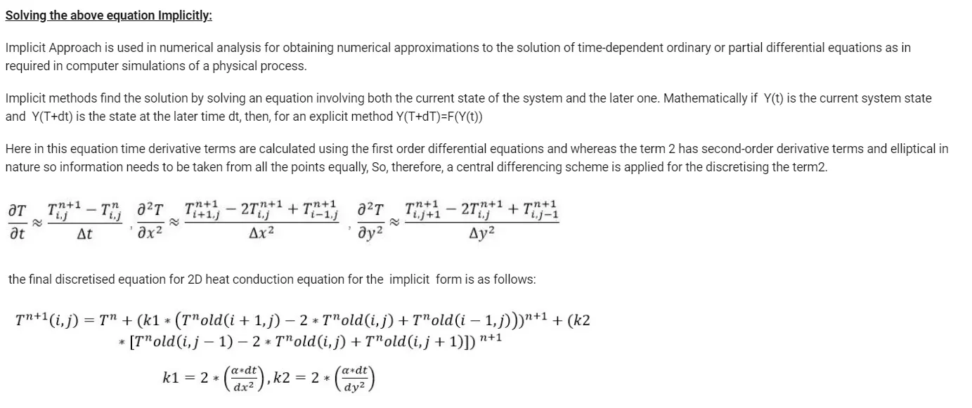
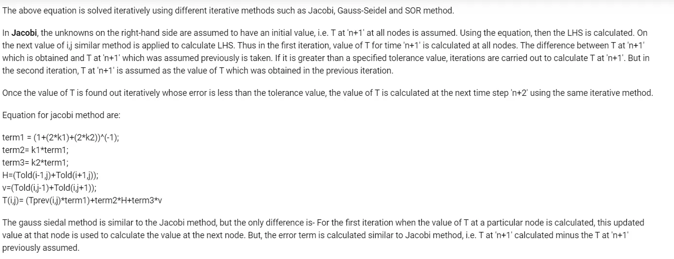
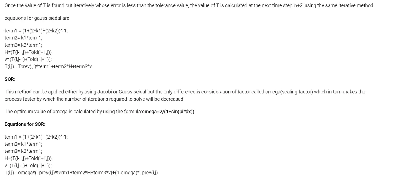
Implicit Tranisent matlab code :

%solving 2D Transient heat conduction equation Implicitly
clear all
close all
clc
%defining the inputs 
nx=10;
ny=nx;
x=linspace(0,1,nx);
y=linspace(0,1,ny);
dx=x(2)-x(1);
dy=y(2)-y(1);
dt=0.1;
%Thermal diffusivity 
diffusivity=0.014;
[xx,yy]=meshgrid(x,y);
%Defining the boundary conditions
T=300*ones(nx,ny);
T(1,:)=600;
T(end,:)=900;
T(:,1)=400;
T(:,end)=800;
%Rounding off the corner values
T(1,1)=(400+600)/2;
T(1,ny)=(600+800)/2;
T(nx,1)=(400+900)/2;
T(nx,ny)=(900+800)/2;
%creating a copy of T
Told=T;
%Tolerance error value and initializing the error value to a random number greater than 1
 tol=1e-4;
 error=500;
 k1=diffusivity*(dt/dx^2);
 k2=diffusivity*(dt/dy^2);
 CFL=k1+k2
 %defining the iterative solvers
 iterative_solver=input('Enter the solver number either 1(jacobi) or 2(Gauss sidel) or 3(SOR) :  ');
 if iterative_solver==1
     tic;
     [T,Convergence_error]=Transient_jacobi_implicit(error,tol,xx,yy,nx,ny,T,k1,k2)
     Time_in_sec=toc
 end
 if iterative_solver==2
     tic;
     [T,Convergence_error]=Transient_gs_implicit(error,tol,xx,yy,nx,ny,T,k1,k2)
     Time_in_sec=toc
 end
  if iterative_solver==3
     tic;
     [T,Convergence_error]=Transient_SOR_implicit(error,tol,xx,yy,nx,ny,T,k1,k2)
     Time_in_sec=toc
 end

Implicit Jacobi function code :

function [T,error]=Transient_jacobi_implicit(error,tol,xx,yy,nx,ny,T,k1,k2)
jacob_iter=1;
Timesteps=1;
Told=T;
%At t=0sec
Tprev=T;

    for q=1:1580 %Time loop for acheiving the steady state solution
        error=500;
        while (error>tol)
        %Space loop for calculation of Temperature at inner nodes except at boundary values for specific time step
    for i=2:nx-1
        for j=2:ny-1
            term1=1/(1+(2*k1)+(2*k2));
            term2=k1*term1;
            term3=k2*term1;
            H=Told(i-1,j)+Told(i+1,j);
            V=Told(i,j+1)+Told(i,j-1);
            T(i,j)=Tprev(i,j)*term1+H*term2+V*term3;
        end
    end  
    %Error for steady state convergence
    error=max(max(abs(Told-T)));
    %Updating the  Temperture values for the calculation of next time steps i.e 0.1,0.2,...........122 sec
    Told=T;
    jacob_iter=jacob_iter+1;
        end
        Tprev=T;
        
figure(1)
    [c,d]=contourf(xx,yy,T);
    colormap(jet)
    colorbar
    set(gca,'ydir','reverse')
    title_text=sprintf('No of timesteps  = %d  for convergence to steadystate',Timesteps);
    title_text1=sprintf('No of Iterations in jacobi  = %d for all time steps',jacob_iter);
    title({'Transient state Implicit method';title_text;title_text1})
    xlabel('xaxis')
    ylabel('yaxis')
    clabel(c,d)
    Timesteps=Timesteps+1;
    end
end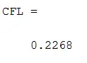

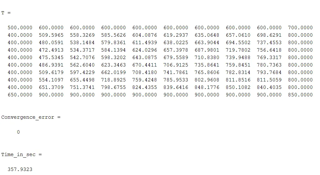
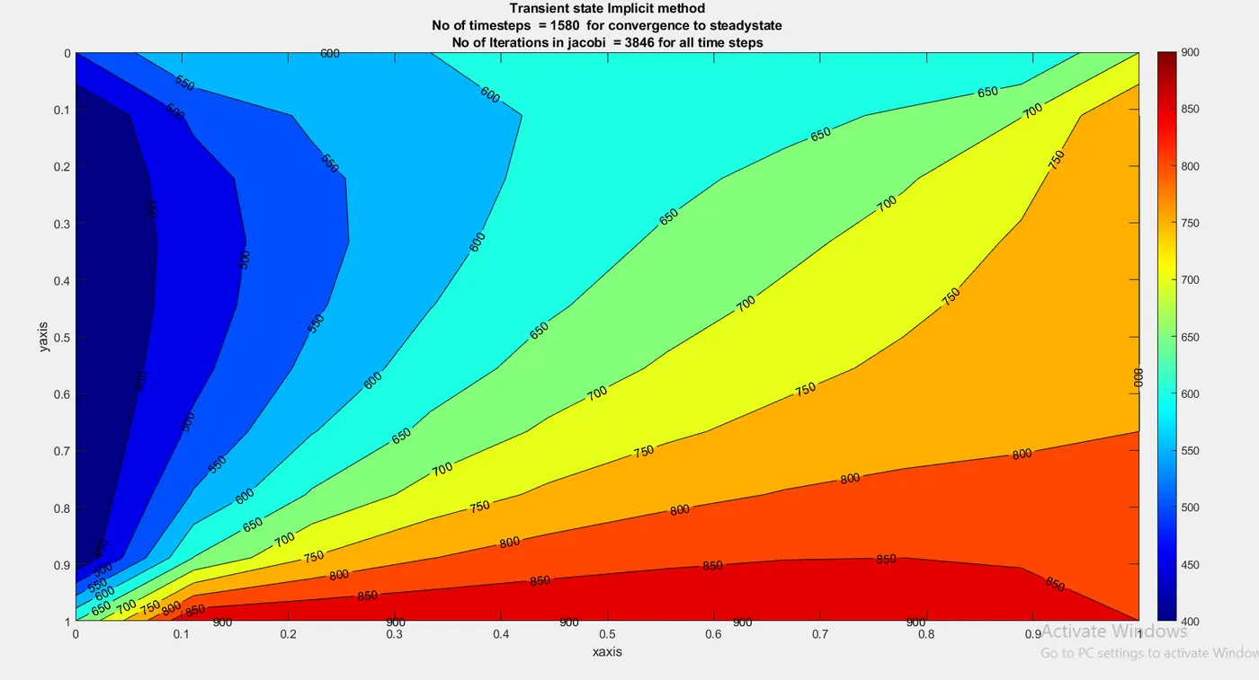
Implicit Gauss siedel function code :

function [T,error]=Transient_gs_implicit(error,tol,xx,yy,nx,ny,T,k1,k2)
gs_iter=1;
Timesteps=1;
Told=T;
%At t=0sec
Tprev=T;

    for q=1:1400 %Time loop for acheiving the steady state solution
        error=500;
        while (error>tol)
        %Space loop for calculation of Temperature at inner nodes except at boundary values for specific time step
    for i=2:nx-1
        for j=2:ny-1
            term1=1/(1+(2*k1)+(2*k2));
            term2=k1*term1;
            term3=k2*term1;
            H=T(i-1,j)+Told(i+1,j);
            V=Told(i,j+1)+T(i,j-1);
            T(i,j)=Tprev(i,j)*term1+H*term2+V*term3;
        end
    end  
    %Error for steady state convergence
    error=max(max(abs(Told-T)));
    %Updating the  Temperture values for the calculation of next time steps i.e 0.1,0.2,...........122 sec
    Told=T;
    gs_iter=gs_iter+1;
        end
        Tprev=T;
figure(1)
    [c,d]=contourf(xx,yy,T);
    colormap(jet)
    colorbar
    set(gca,'ydir','reverse')
    title_text=sprintf('No of timesteps  = %d  for convergence to steadystate',Timesteps);
    title_text1=sprintf('No of Iterations in Gauss sidel  = %d for all time steps',gs_iter);
    title({'Transient state Implicit method';title_text;title_text1})
    xlabel('xaxis')
    ylabel('yaxis')
    clabel(c,d)
    Timesteps=Timesteps+1;
    end
end

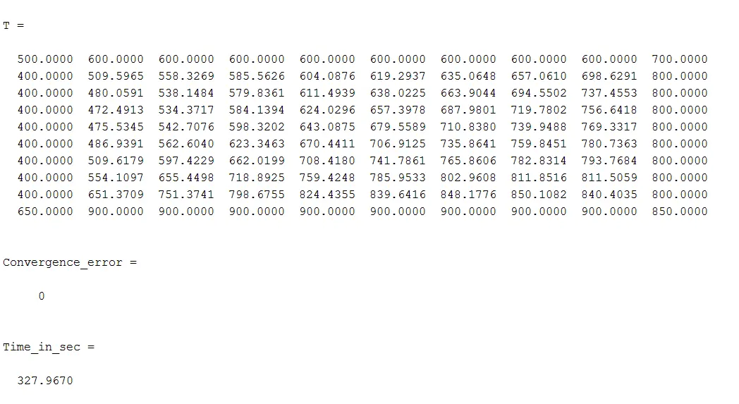
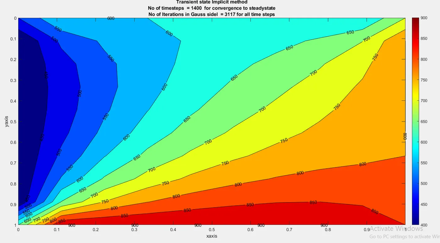
Implicit SOR function code :

function [T,error]=Transient_SOR_implicit(error,tol,xx,yy,nx,ny,T,k1,k2)
SOR_iter=1;
Timesteps=1;
Told=T;
%At t=0sec
Tprev=T;
omega=1.1;

    for q=1:1280 %Time loop for acheiving the steady state solution
        error=500;
        while (error>tol)
        %Space loop for calculation of Temperature at inner nodes except at boundary values for specific time step
    for i=2:nx-1
        for j=2:ny-1
            term1=1/(1+(2*k1)+(2*k2));
            term2=k1*term1;
            term3=k2*term1;
            H=T(i-1,j)+Told(i+1,j);
            V=Told(i,j+1)+T(i,j-1);
            Tgs(i,j)=Tprev(i,j)*term1+H*term2+V*term3;
            T(i,j)=((1-omega)*Told(i,j)+(Tgs(i,j)*omega));
        end
    end  
    %Error for steady state convergence
    error=max(max(abs(Told-T)));
    %Updating the  Temperture values for the calculation of next time steps i.e 0.1,0.2,...........122 sec
    Told=T;
    SOR_iter=SOR_iter+1;
        end
        Tprev=T;
figure(1)
    [c,d]=contourf(xx,yy,T);
    colormap(jet)
    colorbar
    set(gca,'ydir','reverse')
    title_text=sprintf('No of timesteps  = %d  for convergence to steadystate',Timesteps);
    title_text1=sprintf('No of Iterations in SOR  = %d for all time steps',SOR_iter);
    title({'Transient state Implicit method';title_text;title_text1})
    xlabel('xaxis')
    ylabel('yaxis')
    clabel(c,d)
    Timesteps=Timesteps+1;
    end
end

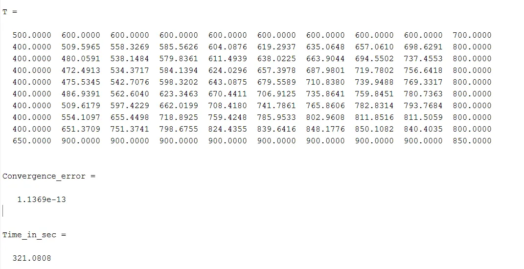
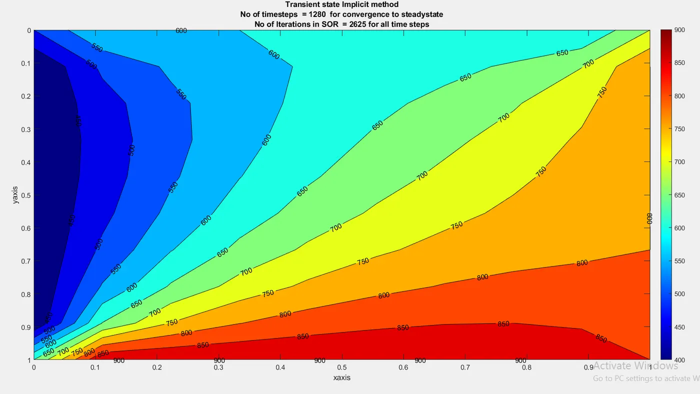
Comparision of the Techniques for Transient state condition :

From the above 3 techniques SOR takes less time and few iterations to converge to the steady state value if a desired omega value is choosen . If omega is too large the solution overshoots and takes more amount of time than jacobian and guass siedel at the same time it should not be too less.

Time SOR < Time GS < Time jacobi

No of iterations in SOR < No of iterations in GS < No of iterations in jacobi