Simulating Fluid Sloshing effect inside a Gear-box
Simulating Fluid Sloshing effect inside a Gear-box
Aim : Simulating the fluid sloshing effect in gearbox and to compare results among these 4 cases shown below
Part 1:
- 20% Immersion, Fluid - Engine oil.
- 30% Immersion, Fluid- Engine oil.
- 20% Immersion,Fluid-n-heptane (c7h16).
- 30% Immersion,Fluid-n-heptane (c7h16).
Part 2:
- What is Dynamic meshing? Give some other examples where dynamic meshing can be used.
- What is the fluid Sloshing effect? Discuss whether the sloshing effect is good or bad? Explain.
- What is the use of UDF?
- Discuss the common errors that occurred in the simulation.
- A] 'Dynamic mesh failed' error.
- B] 'Negative cell volume detected' error.
Introduction :
A typical gearbox consists of some number of gears and gear housing that compositely enables it's purpose. That means that gears are used to transform power by multiplying the out put , the variius components that are used in a typical gear box are shown below as a picture . Gears inside the gear box useully rotate about a prescribed axis ,enhansing the power output . When the gears re rotating in the gear box the friction developed between the two geare is truely high and that leads to a large development of frictional forses and heat . Which may further lead to reduction of life span and performance of gear as well. Inorder to reduce these kind of losses and to increase the power output, we typically use lubricant . More precisely the lubricant is implememented between 2 gears in gear housing . As gears are revolving around their respective axes the lubrucant flud that is present under the gears will also moves accordingly to that . As part of that it may shows some impact on the surroundings this kind of behaviour of fluid is known as sloshing . This can be seen in lot of areas of engineering and science applications where fluid, structure interractions are taking place such as in aircraft , spacecraft etc. In this challenge I simulated a similar kind of case setup of gears along with UDF to control motion of gear that which is been used in industry.
SIMULATION PROCEDURE :
- For this simulation , geometry and meshing steps for all the four cases we are going to be investigated remains same .Once the geometry and meshing has been done , the simulation is performed for different case setups .
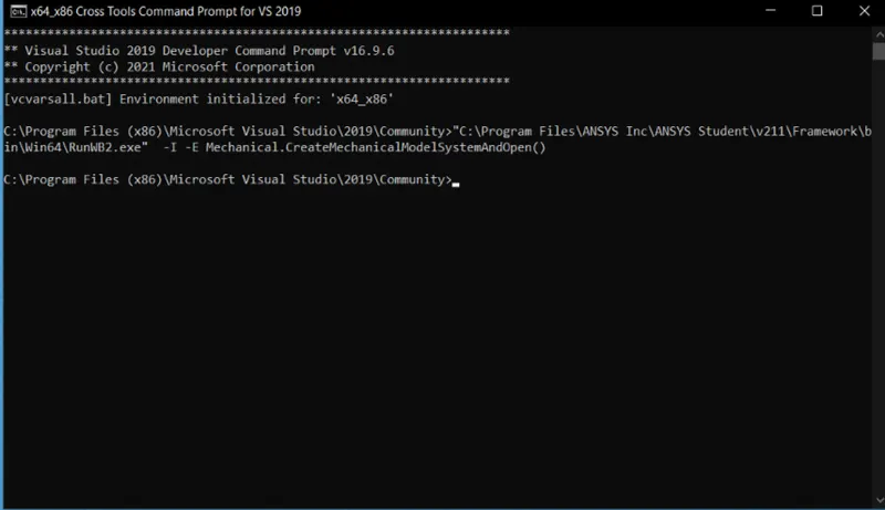
- To define the motion of gears in simulation we are using a user defined function . So as to load in part of the simulation case setup , we should open Ansys from Microsoft Visual C++
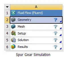
- The simulation workflow that is implemented in this simulation is
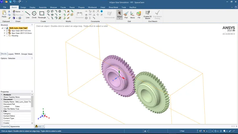
- Geometry of gear box is imported in spaceclaim
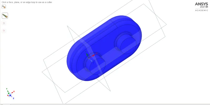
simulation has to be performed in this region . This region is extracted and directly imported in meshing for the meshing operation .
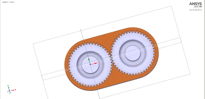
MESHING :
- A base line mesh of element size 30 mm has been developed in ansys meshing
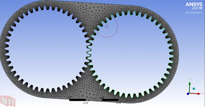
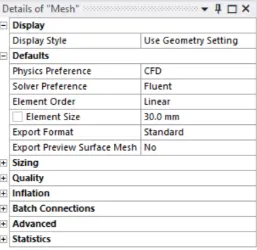
- The generated mesh here is of triangular mesh .
- After meshing for the purpose of giving motion to each gear by matching with the user desined function for gear motion , both gears were given names as left gear and right gear .
- This naming action performed by simply selecting each and every edge mannually by edge selection tool .
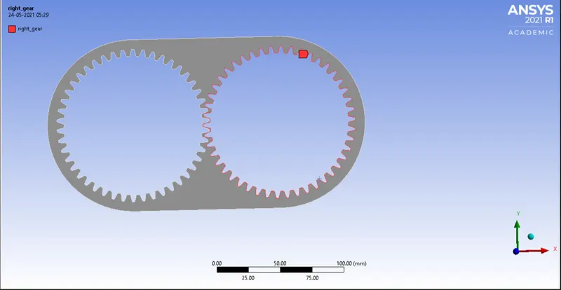
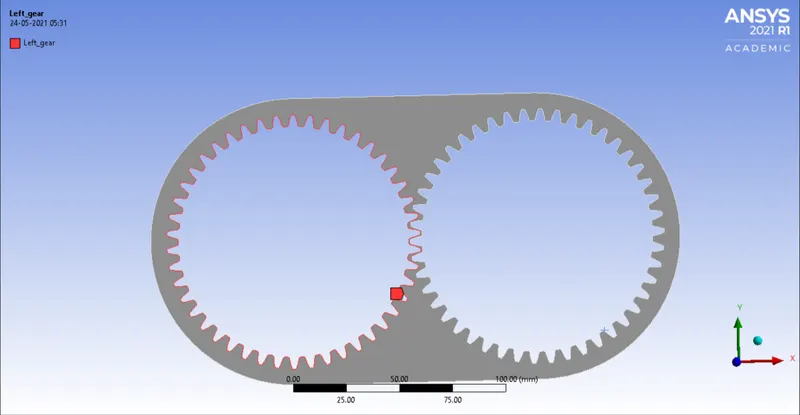
- Now that we are done with fluid region volume extraction and meshing , simulation setup is done through cases in ansys fluent according to the challenge
CASE I : 20% Immersion, Fluid - Engine oil
- Up on moving to ansys fluent for meshing operation, first we need to define the materia that presnt in gear housoing along with air.
- Here in case it is engine oil
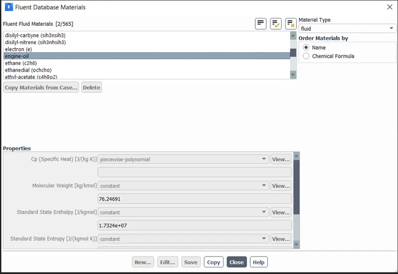
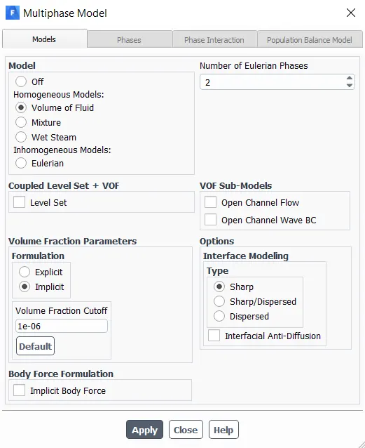
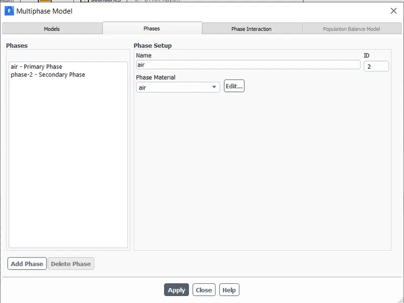
- We are simulating gear sloshing effect ,in this the lubricant and air are going to be interracting with the gears .That means it includes the simulation of materails that are in of 2 different phases .Air is in gas phase and Engine oil is in liquid phase .Hence we need to impliment multiphase model
- We are choosing volume of fluid methods for the simulation of materials of 2 different phases.Volume fraction parameters here is implicit form because if we go for explicit formulation , it leads to exceeding of courant number beyond the limits .In order to limit this , we are using implicit formulation .
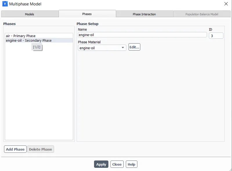
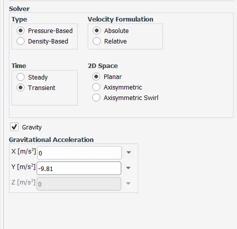
- Solver details :
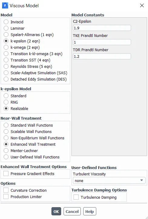
- Viscous model :
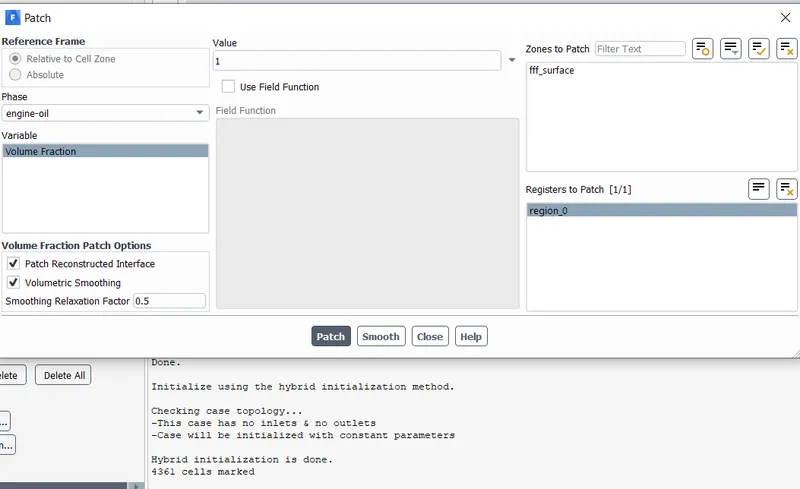
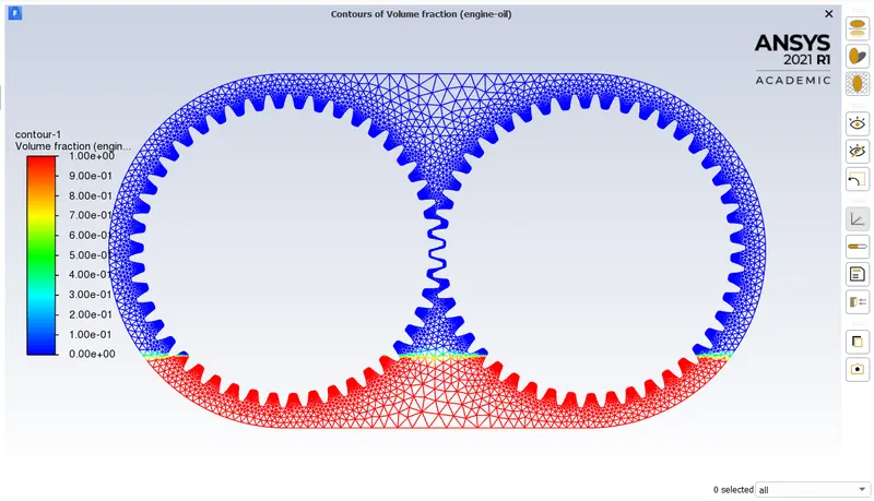
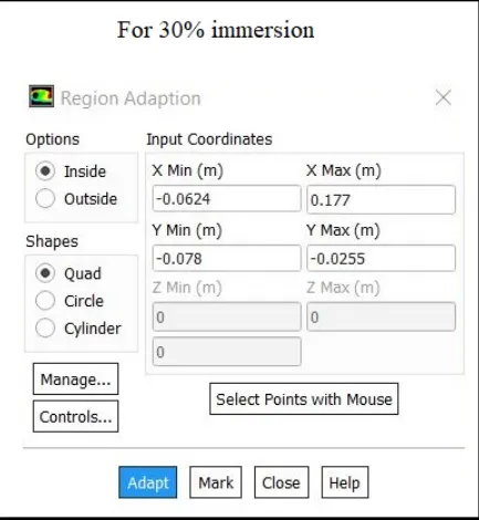
- Now we need to mark the cells according to the required setup.In this case the gears has to be immersed up to 20% of its their volume.
- Upon calculating with respect to the distance between top and bottom surfaces of gear housing the maximum and minimum coordinates of the extremum points are found to be like this
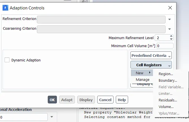
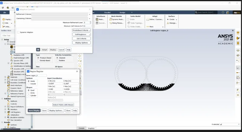
- That black shaded region is the actual lubricant level that is been simulated .
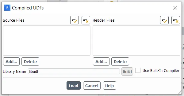
- No we need to load the user defined function in to fluent
-
#include "udf.h" DEFINE_CG_MOTION(right_motion, dt, vel, omega, time, dtime) { vel[0] = 0.0; vel[1] = 0.0; vel[2] = 0.0; omega[0] = 0.0; omega[1] = 0.0; omega[2] = 2.0e2; /* [rad/s]*/ } DEFINE_CG_MOTION(left_motion, dt, vel, omega, time, dtime) { vel[0] = 0.0; vel[1] = 0.0; vel[2] = 0.0; omega[0] = 0.0; omega[1] = 0.0; omega[2] = -2.0e2; /* [rad/s]*/ } 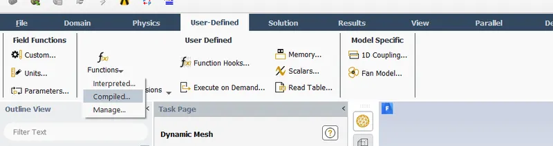
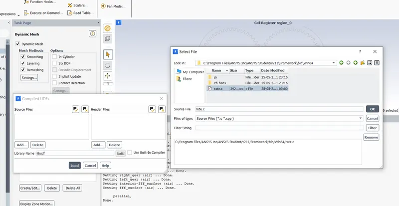
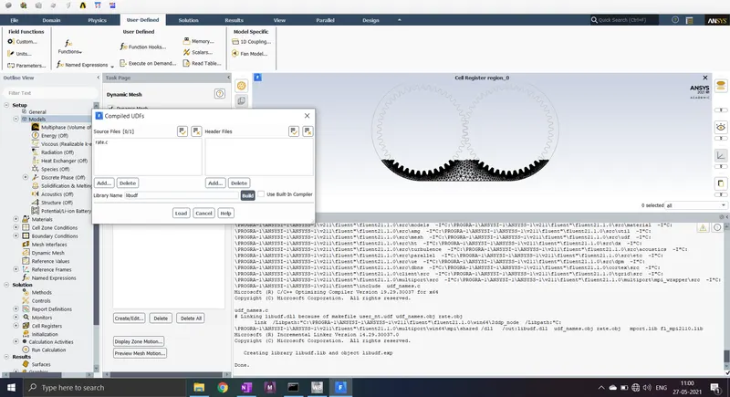
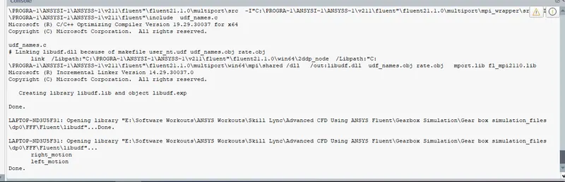
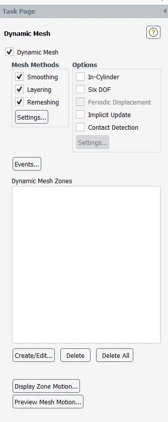
- As we are simulating the moving gears wen need to prepare dynamic mesh .In this part , the mesh is aligned accordingly with the given UDF that describes motion of gears .
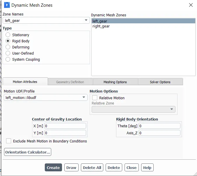
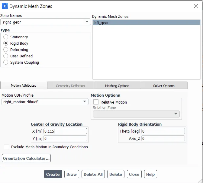
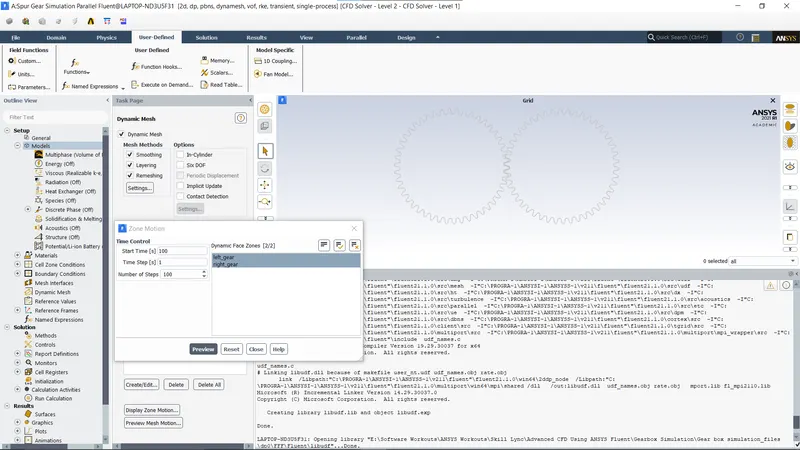
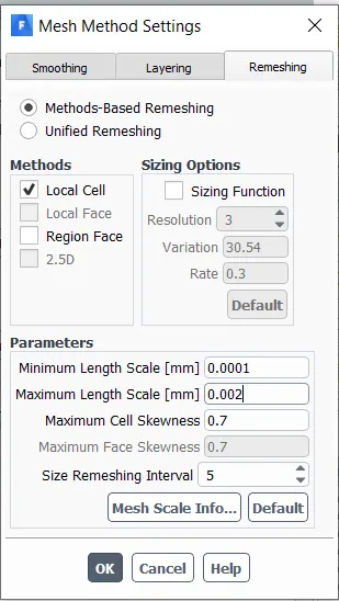
- For the proper calculation of the results ,tmesh method settings play a major role .
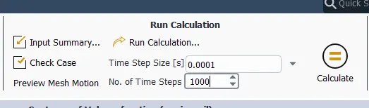
- SOLVING :
- Initialising and patching :
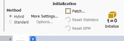
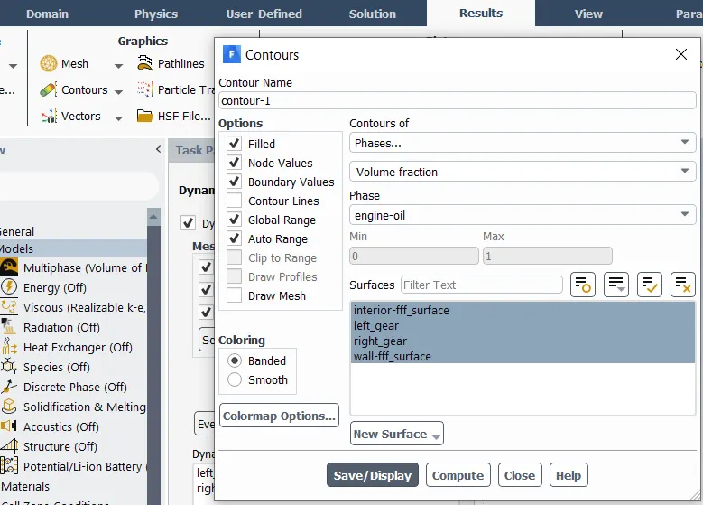
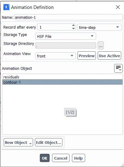
- Contours and animation setting
- RESULTS :
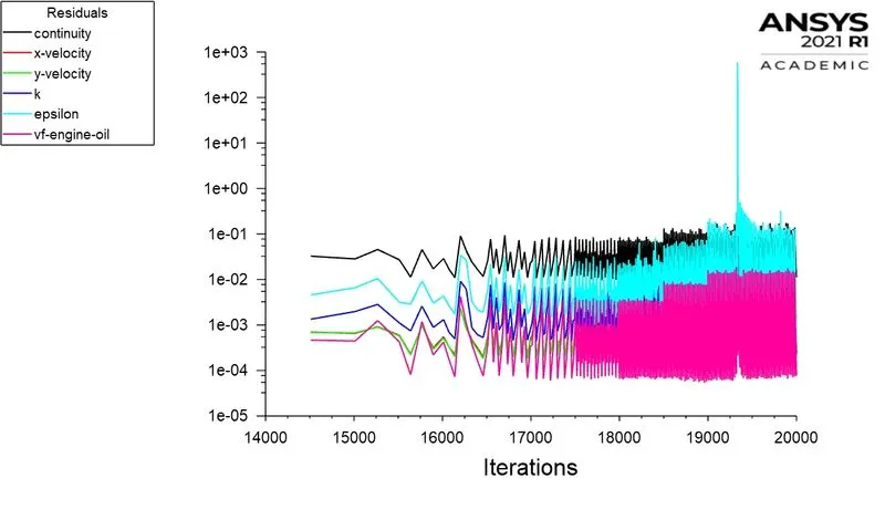
- Residuals :
- Contours :
- M
- Animation :
CASE II -20% Immersion Fluid-n-heptane (c7h16):
- Note : Multi phase setup,solver,viscous,marking cells,UDF,Dynamic meshing,mesh method settings,Initialising will be same as Case -I
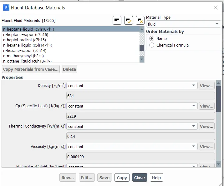
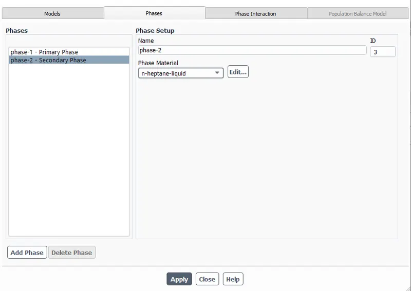
- Material Importing :
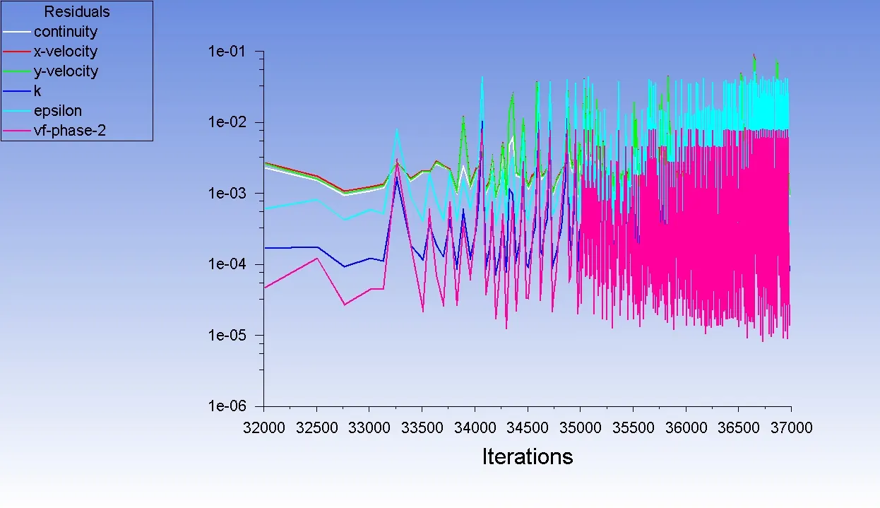
- Animation 20% Immersion Fluid-n-heptane (c7h16) :
- CASE-III 30% Immersion, Fluid- Engine oil.
- Note : Multi phase setup,solver,viscous,,UDF,Dynamic meshing,mesh method settings,Initialising will be same as Case -I
-
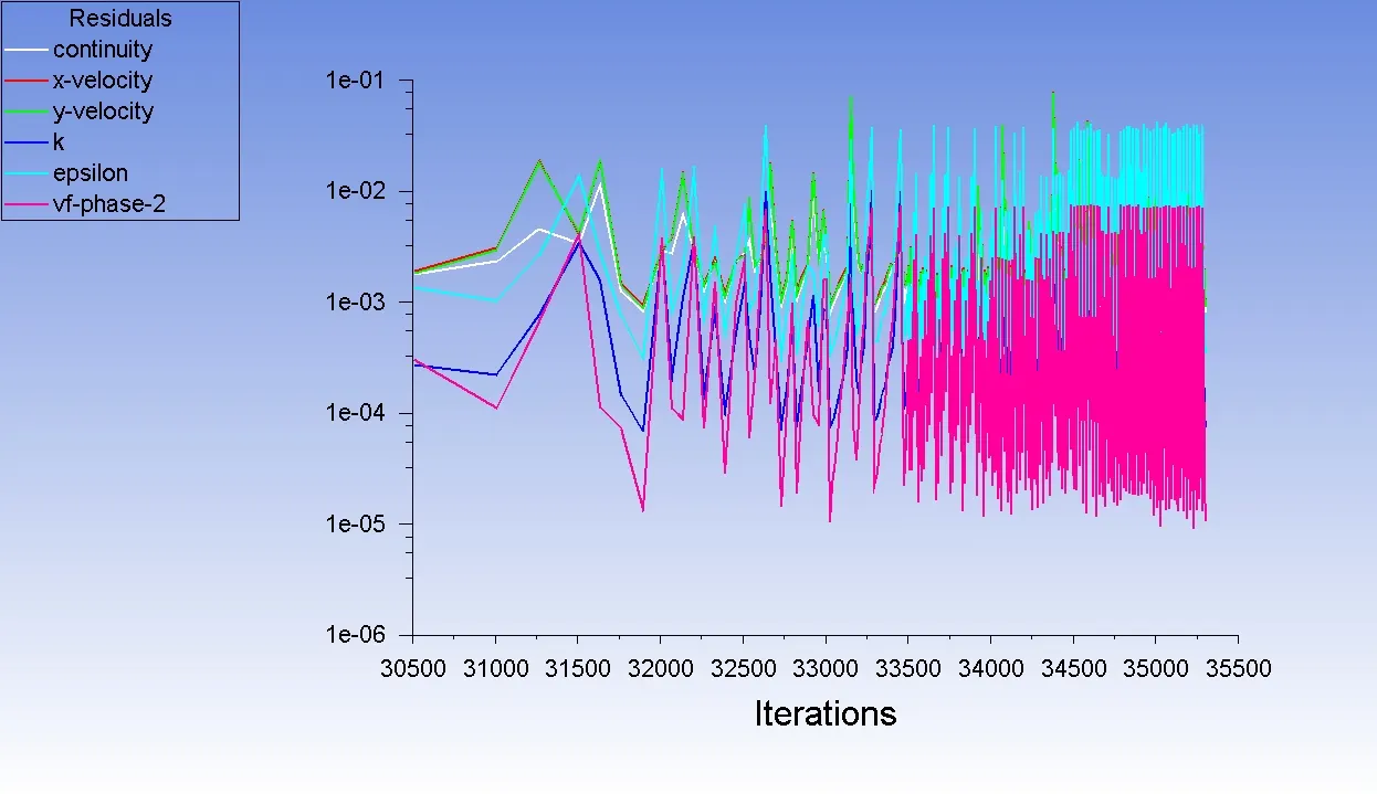
- contours :
- 30% Immersion, Fluid- Engine oil ANIMATION :
CASE-IV 30% Immersion,Fluid-n-heptane (c7h16).
- Note : Multi phase setup,solver,viscous,,UDF,Dynamic meshing,mesh method settings,Initialising will be same as Case -II
- Contours :
30% Immersion,Fluid-n-heptane (c7h16). animation :
Part 2:
Dynamic Meshing- In ANSYS Fluent the dynamic mesh capability is used to simulate problems with boundary motion, such as check valves and store separations.
The dynamic mesh model allows to move the boundaries of a cell zone relative to other boundaries of the zone and to adjust the mesh accordingly. The boundaries can move rigidly with respect to each other (that is, linear or rotational motion). The motion of the boundaries can be rigid, such as pistons moving inside an engine cylinder or a flap deflecting on an aircraft wing, or deforming, such as the elastic wall of a balloon during inflation or a flexible artery wall responding to the pressure pulse from the heart. In either case, the nodes that define the cells in the domain must be updated as a function of time, and hence the dynamic mesh solutions are inherently unsteady.
The building blocks for dynamic mesh capabilities within ANSYS Fluent are three dynamic mesh schemes, namely, smoothing, layering, and remeshing. A combination of these three schemes is used to tackle the most challenging dynamic mesh problems. However, for simple dynamic mesh problems involving linear boundary motion, the layering scheme is often sufficient. For example, flow around a check valve can be simulated using only the layering scheme. The three dynamic mesh schemes are explained below:
1. Smoothing- When smoothing is used to adjust the mesh of a zone with a moving and/or deforming boundary, the interior nodes of the mesh move, but the number of nodes and their connectivity does not change. In this way, the interior nodes “absorb” the movement of the boundary.
2. Layering- The dynamic layering method is used to split or merge cells adjacent to any moving boundary if all cells adjacent to the moving face zone are either wedges or hexahedra (quadrilaterals in 2D) even though the cell zone may contain mixed cell shapes. The cell layers must be completely bounded by one-sided face zones, except when sliding interfaces are used.
3. Remeshing- When the boundary displacement is large compared to the local cell sizes, the cell quality can deteriorate or the cells can become degenerate if only mesh smoothing is used. This will invalidate the mesh (for example, result in negative cell volumes) and consequently, will lead to convergence problems when the solution is updated to the next time step. Hence, for such problems, remeshing is used.
Following are some examples of problems in which dynamic meshing is required which are already mentioned in the above theory:
1. Flow around check valve
2. Pistons moving inside an engine cylinder
3. Flap deflecting on an aircraft wing
4. A flexible artery wall responding to the pressure pulse from the heart.
The dynamic mesh model in ANSYS Fluent can be used to model flows where the shape of the domain is changing with time due to motion on the domain boundaries. The dynamic mesh model can be applied to single or multiphase flows (and multi-species flows). The update of the volume mesh is handled automatically by ANSYS Fluent at each time step based on the new positions of the boundaries. To use the dynamic mesh model, it is required to provide a starting volume mesh and the description of the motion of any moving zones in the model. ANSYS Fluent allows user to describe the motion using either boundary profiles, user-defined functions (UDFs), or the six degrees of freedom solver.
Following are some advantages and disadvantages of dynamic meshing:
Advantages-
1. Its easy to adjust the mesh by moving the boundaries of a cell zone relative to other boundaries of the zone.
2. The boundaries can move rigidly with respect to each other i. e. linear or rotational motion.
3.Mesh zones moving adjacent to one another can be linked across one or more non-conformal interfaces.
Disadvantages-
1. It works efficiently only for the triangular mesh.
2. When the boundary displacement is large compared to the local cell sizes, the cell quality can deteriorate.
3. Convergence problems, when the solution is updated for negative cell volume.
Fluid Sloshing Effect- In fluid dynamics, slosh refers to the movement of liquid inside another object (which is, typically, also undergoing motion).
Strictly speaking, the liquid must have a free surface to constitute a slosh dynamics problem, where the dynamics of the liquid can interact with the container to alter the system dynamics significantly. Important examples include propellant slosh in spacecraft tanks and rockets (especially upper stages), and the free surface effect (cargo slosh) in ships and trucks transporting liquids (for example oil and gasoline). However, it has become common to refer to liquid motion in a completely filled tank, i.e. without a free surface, as "fuel slosh".
Such motion is characterized by "inertial waves" and can be an important effect in spinning spacecraft dynamics. Extensive mathematical and empirical relationships have been derived to describe liquid slosh. These types of analyses are typically undertaken using CFD and FEA to solve the fluid-structure interaction problem, especially if the solid container is flexible. Relevant fluid dynamics non-dimensional parameters include the Bond Number, the Weber number, and the Reynolds number.
Slosh is an important effect for spacecraft, ships, and some aircraft. Slosh was a factor in the Falcon 1 second test flight anomaly, and has been implicated in various other spacecraft anomalies, including a near-disaster with the Near Earth Asteroid Rendezvous (NEAR Shoemaker) satellite.
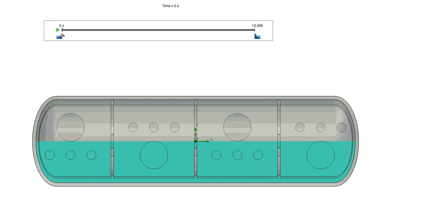
Figure 18. Fuel Tank Sloshing
Whether the sloshing effect is good or bad depends on the application of sloshing. Following are some good and bad applications of sloshing:
Good Application- 1. In gearbox sloshing the movement of viscous liquid is an essential requirement to reduce the temperature and friction losses by providing lubrication to gears. Sloshing is responsible for an increase in the life of the gearbox and its effective working.
2. Use of anti-slosh devices such as baffles to limit the adverse liquid slosh effect on directional performance and stability of tank vehicles.
Bad Application- 1. Liquid sloshing strongly influences the directional dynamics and safety performance of highway tank vehicles in a highly adverse manner. Hydrodynamic forces and moments arising from liquid cargo oscillations in the tank under maneuvers like steering or braking or both simultaneously reduce the stability limit and controllability of partially filled tank vehicles.
UDF- A user-defined function, or UDF, is a function that you program that can be dynamically loaded with the FLUENT solver to enhance the standard features of the code. UDFs are written in the C programming language. They are defined using DEFINE macros that are supplied by Fluent Inc. They access data from the FLUENT solver using predefined macros and functions also supplied by Fluent Inc. Every UDF contains the udf.h file inclusion directive (#include "udf.h") at the beginning of the source code file, which allows definitions for DEFINE macros and other Fluent-provided macros and functions to be included during the compilation process. UDFs are executed as either interpreted or compiled functions in FLUENT. Values that are passed to the solver by a UDF or returned by the solver to a UDF must be specified in SI units.
UDFs allow you to customize FLUENT to fit your particular modeling needs. UDFs can be used for a variety of applications, some of which are listed below:
1. Customization of boundary conditions, material property definitions, surface and volume reaction rates, source terms in FLUENT transport equations, source terms in user-defined scalar (UDS) transport equations, diffusivity functions, etc.
2. Adjustment of computed values on a once-per-iteration basis.
3. Initialization of a solution.
4. Asynchronous execution of a UDF (on demand).
5. Post-processing enhancement.
6. Enhancement of existing FLUENT models (e.g., discrete phase model, multiphase mixture model, discrete ordinates radiation model).
Limitation- Although the UDF capability in FLUENT can address a wide range of applications, it is not possible to address every application using UDFs. Not all solution variables or FLUENT models can be accessed by UDFs. Specific heat values, for example, cannot be modified; this would require additional solver capabilities.
Errors in the Simulation-
A] 'Dynamic Mesh Failed' error- This error occurs due to unsuitable settings of Smoothing, Meshing, and Remeshing. Due to wrong settings of dynamic mesh, the following conditions are not met:
- The boundary of the cell zone moves predominantly in one direction (i.e., no excessive anisotropic stretching or compression of the cell zone).
- The motion is predominantly normal to the boundary zone.
- The faces are triangular (or linear in 2D).
- The faces to be remeshed are all adjacent to moving loops (i.e., moving nodes).
- The faces are on the same face zone, and form an annular (i.e., closed loop).
- The faces are not part of a symmetry or conformal periodic boundary.
Settings that are applied for the dynamic mesh can be observed in Figure 19. In dynamic mesh only smoothing and remeshing were enabled. Layering was not enabled as the geometry was in 2D. The values for smoothing were kept at default. Values for the remeshing were changed for the solution, maximum length scale was set to 1.5 mm (a bit bigger than element size),maximum cell skewness was set to 0.4, and size remeshing interval was set to 2. It is very important to keep the size remeshing interval minimum as for longer intervals the skewness of cell surpasses the maximum skewness value and then cells get collapsed due to which the mesh fails.
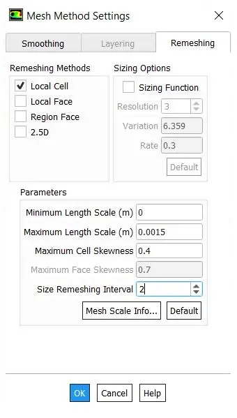
Figure 19. Dynamic Mesh Settings
B] 'Negative Cell Volume Detected' error- Negative cell volume detected error occurs due to the distance moved by a cell per timestep is greater than the cell size in the dynamic region. This problem can be resolved by changing the dynamic mesh settings which are explained above in the 'Dynamic Mesh Fail' error. Another way by which we can resolve the error is by changing the mesh parameters to optimum setting by checking the mesh metrics.
Following are some parameters of mesh metrics used in this simulation to obtain the optimum mesh.
Aspect Ratio: Aspect ratio is the measure of a mesh element's deviation from having all sides of equal length. A high aspect ratio occurs with long, thin elements. Entering an overly large value for the Minimum Element Size mesh control may cause the mesh generator to create solid elements with high aspect ratios. In all triangles method it is always good to keep the value of aspect ratio close to 1 for the better mesh quality.
Element Quality: The Element Quality option provides a composite quality metric that ranges between 0 and 1. This metric is based on the ratio of the volume to the sum of the square of the edge lengths for 2D quad/tri elements, or the square root of the cube of the sum of the square of the edge lengths for 3D elements. A value of 1 indicates a perfect cube, square, or triangle while a value of 0 indicates that the element has a zero or negative volume.
Skewness: Skewness is one of the primary quality measures for a mesh. Skewness determines how close to ideal (equilateral or equiangular) a face or cell is.
The following Table 3 lists the range of skewness values and the corresponding cell quality.
Table 3. Range of Skewness
| Value of Skewness | Cell Quality |
|---|---|
| 1 | degenerate |
| 0.9 — <1 | bad (sliver) |
| 0.75 — 0.9 | poor |
| 0.5 — 0.75 | fair |
| 0.25 — 0.5 | good |
| >0 — 0.25 | excellent |
| 0 | equilateral |
According to the definition of skewness, a value of 0 indicates an equilateral cell (best) and a value of 1 indicates a completely degenerate cell (worst). Degenerate cells (slivers) are characterized by nodes that are nearly coplanar (colinear in 2D).
Highly skewed faces and cells are unacceptable because the equations being solved assume that the cells are relatively equilateral/equiangular.
Conclusion :
- It is observed that the formation of engine oil lubricant film over a gear tooth is more stable than n-heptane as a lubricant on it.
- Sloshing effect is more in the lubricant which will have lower viscosity.
- In this simulation , we can say that Viscosity of n-heptane( 0.000409 kg/m-s) << Viscosity of engine oil(1.06 kg/m-s) .
- As we observed in the cases n-heptane sloshed everywhere unlike the engine oil .This is because n-heptane has less viscosity when compared with engine oil.