Week 3 - Simulating a 2nd order ODE system of a simple pendulum

Theory and Governing Equation:

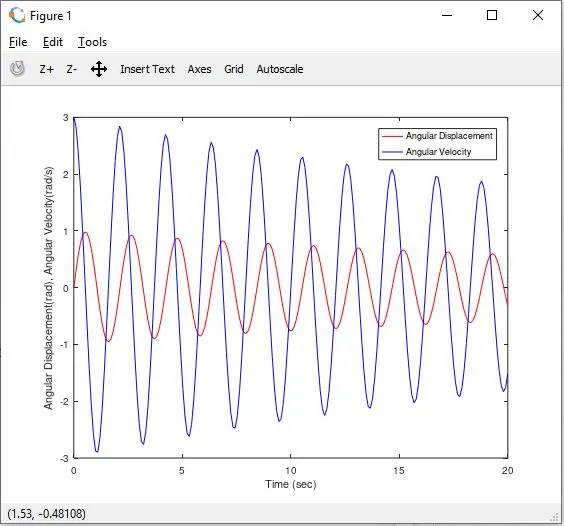
A simple pendulum consists of a point mass m hanging on a string of length L. It is then pulled upto some initial angle `theta` radians and allowed to oscillate freely under the influence of gravity. At the extreme end points, the angular velocity is 0 and angular displacement is maximum whereas at the exactly vertically downwards point the displacement is zero and angular velocity is maximum. Due to frictional effect the oscillations slowly die down which is controlled by the damping coefficient. The motion of the pendulum is governed by the following equation:

`(d^2theta)/(dt^2)+b/m(d theta)/(dt)+g/lsin theta=0`

Logic used to solve the ODE:

As we can only solve first order ODEs in Matlab, so we will try to re-write this second order ODE as a set of 2 first order ODE by using two variables. Here we will assume that `theta1` is `theta`, which is essentially angular displacement and the derivative of `theta1` with respect to time is `theta2`, which is essentially angular velocity. And further the derivative of `theta2` with respect to time is the angular acceleration.

Angular Displacement: `theta =theta1`

Angular Velocity: `theta2=(d theta1)/dt=(d theta)/dt` ---- (1)

Angular Acceleration: `(d theta2)/dt=(d^2theta1)/dt^2=(d^2theta)/dt^2`

We can now re-write the second order ODE as a first order ODE:

`(d^2theta1)/dt^2=-b/m(d theta1)/dt-g/l sin theta1`

`(d theta2)/dt=-b/m theta2-g/lsin theta1` ---- (2)

Equations 1 and 2 are two first order ODEs. Solving them with appropriate boundary conditions will give us angular displacement and angular velocity as a function of time. We need to solve for `theta1` and `theta2`.

`[[(d theta1)/dt], [(d theta2)/dt]]=[[theta2],[-b/m theta2-g/l sin theta1]]`

Explanation of Code:

1. Initially we assign the time interval and divide it into 200 parts and also enter the initial condition of angular displacement and angular velocity at time t=0.
2. Next we will define a function that contains the two first order ODEs, solving which we will get the angular displacement and angular velocity as a function of time.
3. Now we will call the above function and solve the pair of first order ODEs using ode45 function.
4. Then we will plot the angular displacement and angular velocity plots with time in figure 1.
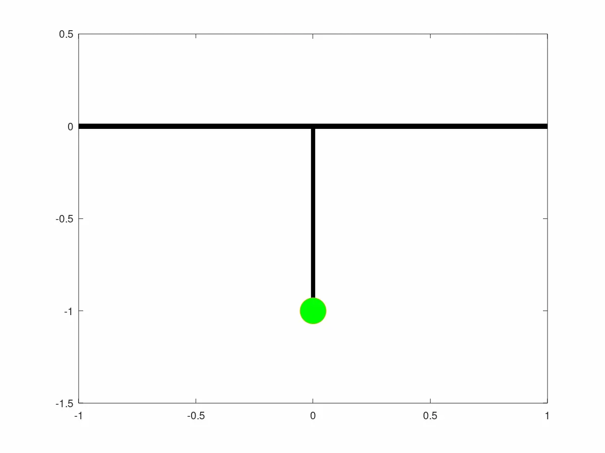
5. After this we will open a figure window 2 and in this we will show the motion of pendulum by using for loop. In each iteration of for loop for a particular value of 'i', we will use the angular displacement value(angle in radians) at that index and locate the position of the bob of pendulum using sin and -cos of that angle.
6. Two lines have been plotted to show the ceiling and rod of pendulum and hold value is kept on so that these lines do no disappear. A green circle ('o') has been drawn to show location of bob. At the end of the for loop, the hold value is changed to off so the current image of pendulum is removed and a new one can be plotted. A pause interval of 0.005 sec has been introduced so that used can see the figure.
7. All the above images are then combined into a single animation(GIF) using imwrite function by appending each new image to the previous ones. The delay time between each image in animation is set to 0.005 and the image is in RGB format.

MATLAB Code:

clear all
close all
clc

t=linspace(0,20,200); %Time interval 0 to 20 seconds divided into 200 parts
theta0=[0,3]; %Initial value of angular displacement(0) and angular velocity(3)

%function containing the two first-order ODE and other parameters describing the motion of pendulum
function [dtheta] = pendulum(t,ans)
  b=0.05;
  m=1;
  g=9.81;
  L=1;
  dtheta=zeros(2,1);
  dtheta(1)=ans(2);
  dtheta(2)=(-b/m)*ans(2)-(g/L)*sin(ans(1));
endfunction

%Calling the function to solve the ODE
[t,ans]=ode45('pendulum',t,theta0);

%plotting the variation of angular displacement and angular velocity with time
figure(1)
plot(t,ans(:,1),'r',t,ans(:,2),'b')
legend('Angular Displacement','Angular Velocity')
xlabel('Time (sec)'), ylabel('Angular Displacement(rad), Angular Velocity(rad/s)')
title('Angular Displacement and Angular Velocity of Pendulum with time')

%plotting position of pendulum at different time and combining them to make animation
figure(2)
for i=1:length(t)
  x=sin(ans(i,1));
  y=-cos(ans(i,1));
  plot([-1,1],[0,0],'linewidth',5,'color','k');
  line([0 x],[0 y],'linewidth',4,'color','k');
  hold on;
  plot(x,y,'o','markersize',25,'markerfacecolor','g');
  axis([-1 1 -1.5 0.5]);
  pause(0.005);
  img = print('-RGBImage');
  imwrite(img,'animation.gif','DelayTime',.005,'Compression','bzip','WriteMode','Append');
  hold off;
end

Angular Displacement and Angular Velocity plot with time:

Animation Video (GIF):