Simulate an animation for the Simple Pendulum using PYTHON

Objective: -

Develop a program that solves the following ODE which represents the equation of motion of a simple pendulum with damping and simulate an animation for the simple pendulum.

Principle: -

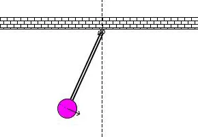
The pendulum moves depend on Newton's second law. When this law is written down, we get a second order Ordinary Differential Equation that describes the position of the "ball" w.r.t time. A simple pendulum consists of a mass m hanging from a string of length L and fixed at a pivot point P. When displaced to an initial angle and released, the pendulum will swing back and forth with the periodic motion. By applying Newton's second law for rotational systems, the equation of motion for the pendulum may be obtained.

Solution procedure: -

ODE represents the equation of motion of a simple pendulum with damping

`(d^2θ)/(d^2t)+b/m*dθ/dt+g/L*sinθ=0`

In the above equation,

g = gravity in m/s2,

L = length of the pendulum in m,

m = mass of the ball in kg,

b=damping coefficient.

we used,

L=1 metre,

m=1 kg,

b=0.05.

g=9.81 m/s2.

Simulation of the motion is done between 0-20 sec, for angular displacement=0,angular velocity=3 rad/sec at time t=0.

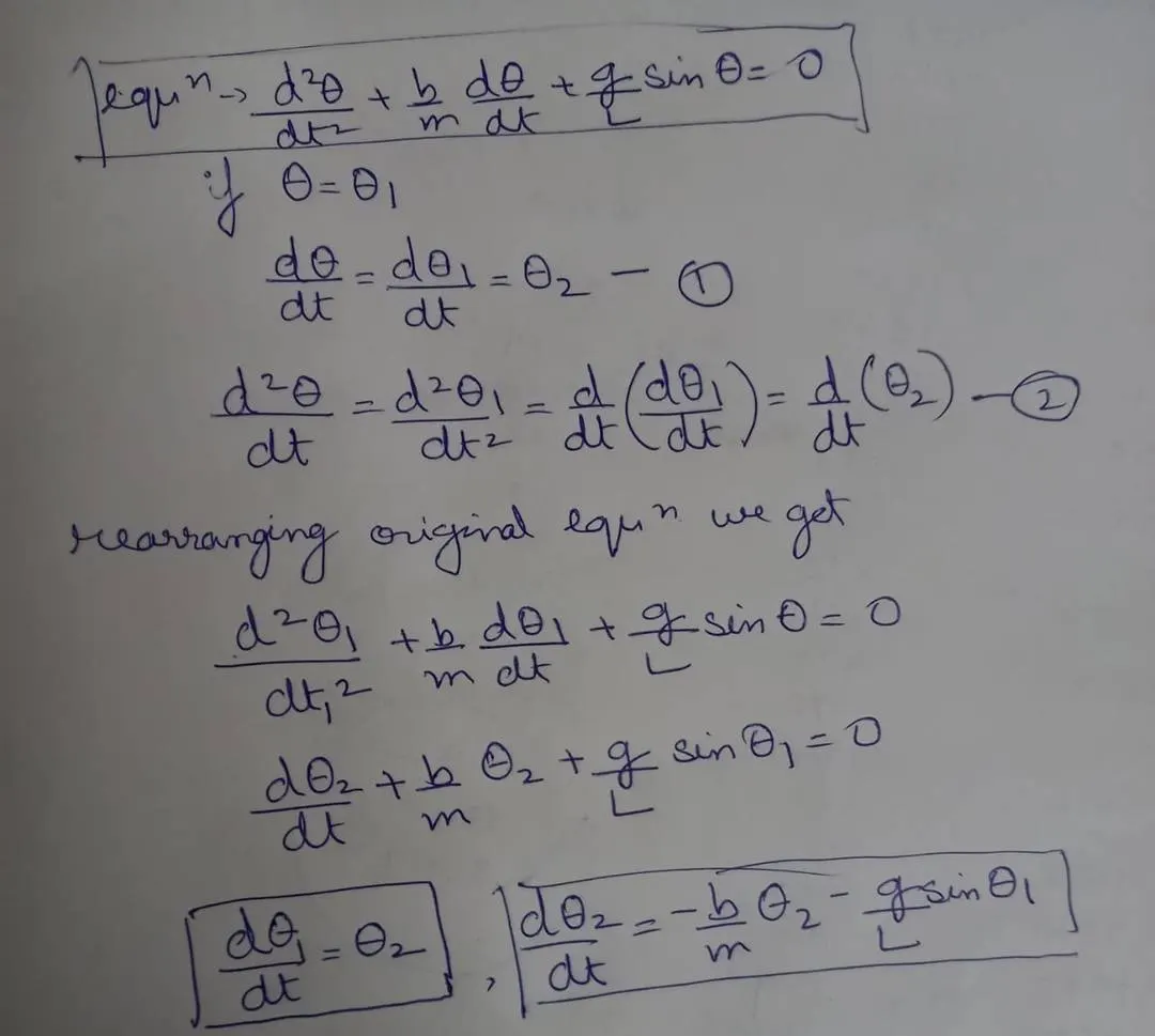
CODE for the function used: -

#defing function returs dz/dt

def model(theta,t,b,g,l,m):

	theta1 = theta[0]
	theta2 = theta[1]
	dtheta1_dt = theta2
	dtheta2_dt = -(b/m)*theta2 - (g/l)*math.sin(theta1)
	dtheta_dt = [dtheta1_dt,dtheta2_dt]
	return dtheta_dt

Explanation of the above code: -

• #defing function returs dz/dt - comments to make a program user friendly
• def model(theta,t,b,g,l,m): - function is used to make the code easy to implement ,it is a group of statements that together perform a task
• theta1 = theta[0]
• theta2 = theta[1]
• dtheta1_dt = theta2 - initializing according to the equation
• dtheta2_dt = -(b/m)*theta2 - (g/l)*math.sin(theta1) - calculating dheta2/dt
• dtheta_dt = [dtheta1_dt,dtheta2_dt]
• return dtheta_dt - to return a value to the calling function

CODE for the animation of a simple pendulum and solving the equation for second order ode: -

import numpy as np
from scipy.integrate import odeint
import matplotlib.pyplot as plt
import math

#defing function returs dz/dt

def model(theta,t,b,g,l,m):

	theta1 = theta[0]
	theta2 = theta[1]
	dtheta1_dt = theta2
	dtheta2_dt = -(b/m)*theta2 - (g/l)*math.sin(theta1)
	dtheta_dt = [dtheta1_dt,dtheta2_dt]
	return dtheta_dt

b=0.05
g=9.81
l=1
m=1

#intial condition
theta_0 = [0,3]

#time points
t=np.linspace(0,20,500)

#solve ODE

theta = odeint(model,theta_0,t,args= (b,g,l,m))

#plot results
plt.plot(t,theta[:,0],'b-',label = r'$frac{dtheta_1}{dt}=theta2$')
plt.plot(t,theta[:,1],'r--',label = r'$frac{dtheta2}{dt}=-frac{g}{L}sintheta_1$')
plt.ylabel('Plot')
plt.xlabel('Time')
plt.legend(loc ='best')
plt.show()

#Animation for simple pendulum
ct=1
for i in  theta[:,0]:
	x0=0
	y0=0
	x1=(l*math.sin(i))
	y1=-(l*math.cos(i))
	filename = 'test%05d.png' % ct
	ct=ct+1

	#Plotting

	plt.figure()
	#Plotting the base line of the pendulum
	plt.plot([-0.5 ,0.5],[0,0],linewidth =5,color ='r')
	plt.plot([x0,x1],[y0,y1],linewidth=3,color = 'g')
	
	plt.plot(x1,y1,'o',markersize =20,color ='black')
	plt.xlim([-1.5,1.5])
	plt.ylim([-1.5,1.5])
	plt.title('Animation of Simple pendulum')
	plt.savefig(filename)

Explantion of the above code: -

• import numpy as np - importing the numpy library to solve numbers in python
• from scipy.integrate import odeint - used to solve Differential equations in Python
• import matplotlib.pyplot as plt - importing mathplot library for plotting the graph
• import math - importing math library to do math operation
• b=0.05 - initializing damping coefficient
• g=9.81 - initializing gravity as 9.81m/s
• l=1 - intializing length of the pendulum as 1 m
• m=1 - initializing mass of the ball as1 kg

#intial condition - comments to make a program user friendly

• theta_0 = [0,3] - initializing the column of theta1 and theta2 as 0 and 3 angular displacement=0,angular velocity=3 rad/sec

#time points - comments

• t=np.linspace(0,20,500) - for simulation of the motion between 0-20 sec , linspace is used to generate 500 values between 0 and 20

#solve ODE - comments

• theta = odeint(model,theta_0,t,args= (b,g,l,m)) - odeint is a command in scipy module it is a function to integrate ordinary differential equation

#plot results - comments

• plt.plot(t,theta[:,0],'b-',label = r'$frac{dtheta_1}{dt}=theta2$') - commant to plot the legend
• plt.plot(t,theta[:,1],'r--',label = r'$frac{dtheta2}{dt}=-frac{g}{L}sintheta_1$') - commant to plot the legend
• plt.ylabel('Plot') - to label the y axis
• plt.xlabel('Time') - to label the x axis
• plt.legend(loc ='best')
• plt.show() - to show the plot

#Animation for simple pendulum - comments

• ct=1 - to initialize ct as 1
• for i in theta[:,0]: - for executing the for loop till the displaceent value in the array
• x0=0 - initializing x0 as 0
• y0=0 - initializing y0 as 0
• x1=(l*math.sin(i)) - initializing x1 coordinate value
• y1=-(l*math.cos(i)) - initializing x2 coordinate value
• filename = 'test%05d.png' % ct -giving the filename as 00001,00002 in sequence order
• ct=ct+1 - incrementing the ct value to give more frames

#Plotting

• plt.figure()

#Plotting the base line of the pendulum

• plt.plot([-0.5 ,0.5],[0,0],linewidth =5,color ='r') - plotting of the baseline of the pendulum
• plt.plot([x0,x1],[y0,y1],linewidth=3,color = 'g') - plotting the string of the pendulum attach to ball
• plt.plot(x1,y1,'o',markersize =20,color ='black') - plotting the bob of the pendulum
• plt.xlim([-1.5,1.5]) - giving the x limit
• plt.ylim([-1.5,1.5]) - giving the y limit
• plt.title('Animation of Simple pendulum') - giving the title to the frames generated
• plt.savefig(filename) - save the frames generated as filename

Output plot: -

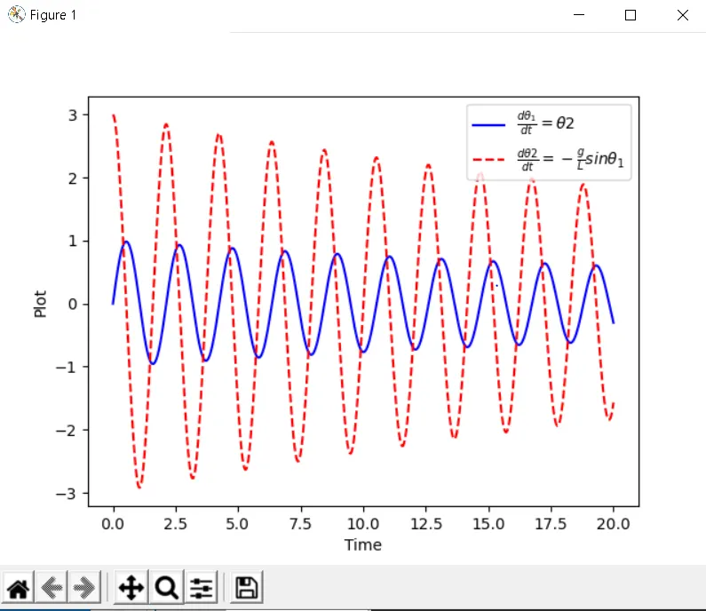
In the above plot blue line shows the displacement and red line shows the velocity both are continuously decreasing due to damping coefficient

Error faced while developing the code: -

• error raised for an Invalid expression.

On debugging it was found out that instead of from scipy import scipy was used

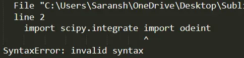
• An error was found because of an indention error in the function

On debugging it was found it was due to an indention problem

• An error was caused due to invalid syntax

On debugging it was found to be (,) was missing

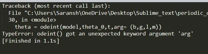
• An error was caused for the invalid keyword

It was found due to the args keyword arg was written

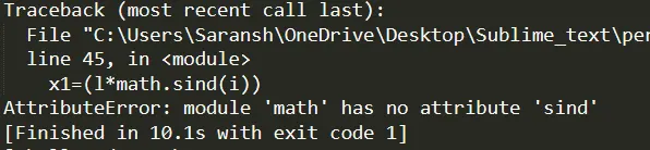
• An error was arisen due to the use of sind and cosd

It was found that the error was neutralized by using sin and cos instead of sind and cosd

Youtube Link for the Animation: -

https://youtu.be/0-onaJxueZg

Conclusion and Discussion: -

• Images generated were saved in a folder and then they were stitched by image magick software and then a gif was created of it and converted to the video and uploaded to youtube.