Shock tube simulation project

Aim:

The major objective of this project was to set up Transient Simulation in a Shock Tube using Converge CFD. A shock tube that has a diaphragm in between and the tube is one side filled with high-pressure Nitrogen where the other side is filled with low-pressure Oxygen.

Introduction

The report contains a detailed description of the Shock tube Simulation problem using converge CFD software, solving it using CYGWIN, and post-processing the result using ParaView. This Case Study contains a rectangular duct that has two sections along with a diaphragm in between. A high-pressure reservoir is connected to the low-pressure section

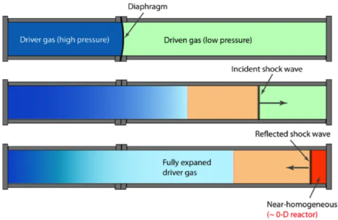
A shock tube is a device for studying shock waves. Prior to starting an experiment, a diaphragm inside the tube blocks any flow. we can increase the pressure on one side, such as with a compressor, and then start the flow by rupturing the diaphragm. The gas expands down the other half of the tube.

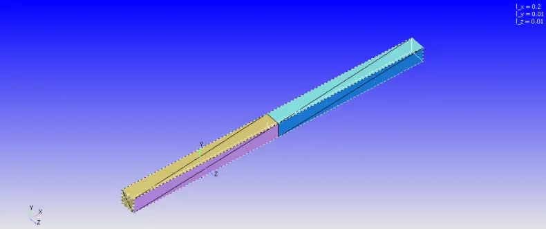
Geometry Creation

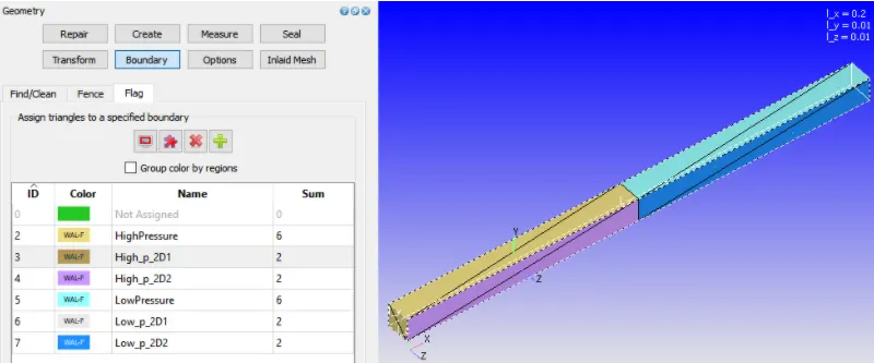
Boundary Creation

Simulation Result

Mesh

Inference:

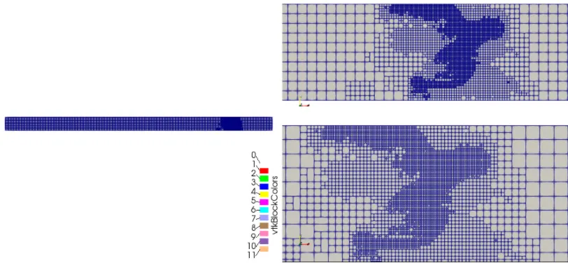
• The above animation of the mesh generation shows how the mesh refinement takes place as the simulation proceeds.
• It can be concluded that the mesh-refinement is done in and around the contact surface in order to capture the variations taking place in this location in far clear manner.

Result:

• Thus, the transient shock tube simulation has been done and the inferences derived.

Contours

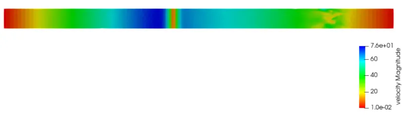
Velocity Contour

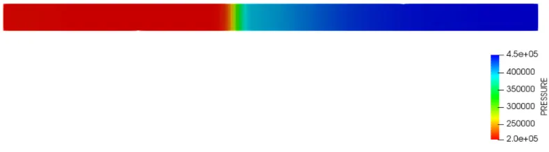
Pressure Contour

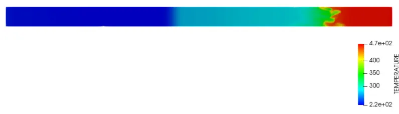
Temperature Contour

The links of the youtube videos for the animations are-

https://youtu.be/fCMR7SiNEkM

https://youtu.be/ka5RM-OnbNA

https://youtu.be/bgLIZTDO1o4

Animation of Velocity variation in Shock tube:

• Observation:
  • The above shows the variation of velocity in the shock tube.
  • The variation in velocity is very drastic all over the domain.
• Inference:
  • The drastic variation in velocity is attributed to the formation of the shock wave.
  • There is no considerable change in velocity of the gases near the ends, which denotes that the gases are at rest at these locations.

Animation of Temperature variation in Shock tube:

• Observation:
• The above shows the variation of temperature in the shock tube.
• There is smooth variation in a particular section and drastic in some sections.

• Inference:
  • The drastic variation in temperature is attributed to the formation of the shock wave.
  • The contact surface and its motion can be identified clearly from the above contour by means of the temperature discontinuity prevailing in the contour in the rightward of the tube. As the shock wave cause drastic increase in the temperature as it passes by, the contact surface is found to have completely different projections of temperature than the other regions.

Plots

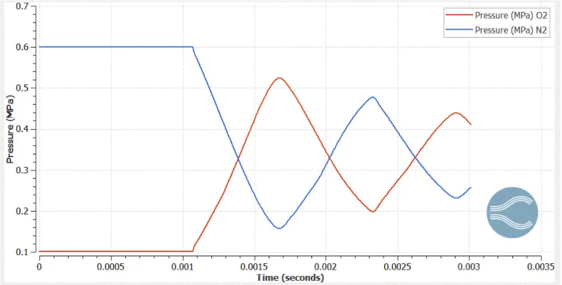
Pressure Plot

• Observation:
  • The pressure is constant until 0.0011s and it varies in cyclic manner as the flow furthers.
  • The amplitude and wavelength of the pressure curve decreases gradually as the simulation continues.
• Inference:
  • The pressure is constant until the diaphragm is closed.
  • As the diaphragm ruptures the average pressure over the entire domain first decreases as the high pressure side mixes with the low pressure side and the shock wave travels towards the low pressure side in addition to expansion wave travelling towards the high pressure side reducing the pressure there.
  • Then it increases as the shock wave travels towards the high pressure region and rises the pressure furthermore. This continues till the simulation ends.
  • Moreover, this would reach a steady state(equillibrium state) if the simulation continues further beyond this time frame.

Temperature Plot

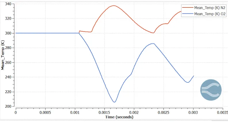
• Observation:
  • The temperature is constant until 0.0011s and it varies in cyclic manner similar to that of pressure.
  • The amplitude and wavelength of the temperature curve decreases gradually as the simulation continues.
• Inference:
  • The temperature also varies in the same fashion as that of the pressure curve.
  • The same reasons are accounted for this too.

Cell Count

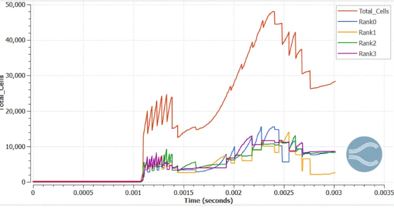
Inference:

• The total number of cells is lesser in the beginning until 0.0011s.
• It increases to a very high number after that. This is because the species AMR feature is enabled only after 0.001s. With the influence of this feature the meshing is made autonomous.
• In species AMR, the N2 is selected, which means that the critical areas of N2 are refined upon satisfaction of a particular condition after 0.001s.
• This leads to the above non-linear change in the number of cells as the simulation progresses.