Project - Speed Control of a Direct Current (DC) motor

Designing PID Controller for desire motor of speed: -

A DC motor is defined as a class of electrical motors that convert direct current electrical energy into mechanical energy.

Motor Schematic Diagram

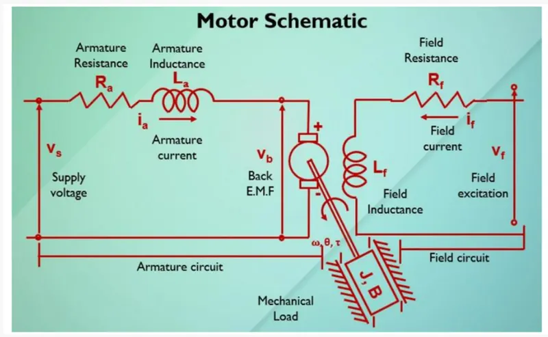
Mathematical modelling from the first principles

Using Kirchhoff’s Voltage Law,

Vs = Ra*ia + La*d(ia)/dt + Vb

Here,

• Vs = Supply Voltage
• Ra = Armature Resistance
• Ia = Armature Current
• La = Armature Inductance
• Vb = Back EMF
• Km = Back EMF constant
• T = Torque
• Kt = Torque constant
• The relation between the Back EMF, angular velocity & Torque are related by
  • Vb = Km*d(theta)/dt, d(theta)/dt = angular velocity
  • T = Kt*Ia.

• The open loop transfer function for the motor with speed(W) & supply voltage (Vs) can be derived as:
  • W(s)/Vs = Kt / [(J *La *s^2) + (J*Ra + B*La) *s+ (B*Ra + Kt*Km)]

• A PID (Proportional Integral & Derivative) controller design to obtain desired angular speed using the supply voltage.

Creating DC_Motor_Parameters.m file in MATLAB

%The design parameters to model a DC motor

J = 0.01; %Moment of inertia of the rotor in kg-m^2

B = 0.1; %Motor Viscous friction constant in N-m-s

Km = 0.01; %Back EMF constant in V/rad/s

Kt = 0.01; %Motor torque constant in N-m/amp

Ra = 1.0; %Resistance of the armature circuit in ohms

La = 0.5; %Inductance of the armature circuit in henrie

% finding matrix A and B

A = [-B/J Kt/J;-Km/La -Ra/La]; % A Matrix

Bm = [0;1/La]; % B Matrix

% parameters for pole design

zeta = 0.89;

fn = 1.0;

wn = 2*pi*fn;

p1 = -zeta*wn+wn*sqrt(zeta^2-1);

p2 = -zeta*wn-wn*sqrt(zeta^2-1);

P = [p1;p2];

% pole placement Design

K = place(A,Bm,P);

Kp = K(1);

Kd = K(2)

Ki = 50;

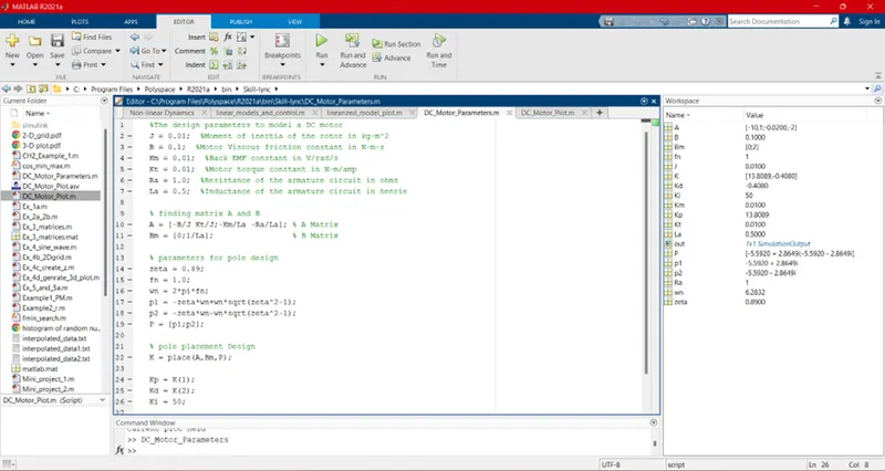
System considers for zeta = 0.89 (more damped system)

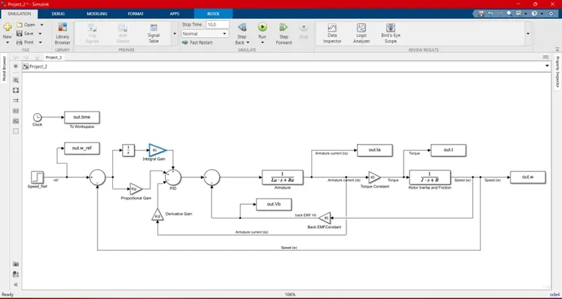
Now, Plotting workspace block graph (‘w_ref’,’Ia’,’Vb’,’t’,’w’)

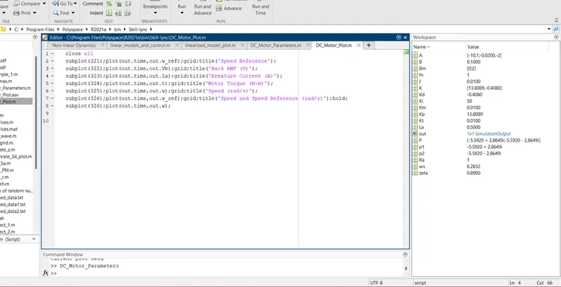
For this another m-file creating using: - edit Dc_Motor_Plot.m

close all
subplot(321);plot(out.time,out.w_ref);grid;title('Speed Reference');
subplot(322);plot(out.time,out.Vb);grid;title('Back EMF (V)');
subplot(323);plot(out.time,out.Ia);grid;title('Armature Current (A)');
subplot(324);plot(out.time,out.t);grid;title('Motor Torque (N-m)');
subplot(325);plot(out.time,out.w);grid;title('Speed (rad/s)');
subplot(326);plot(out.time,out.w_ref);grid;title('Speed and Speed Reference (rad/s)');hold;
subplot(326);plot(out.time,out.w);

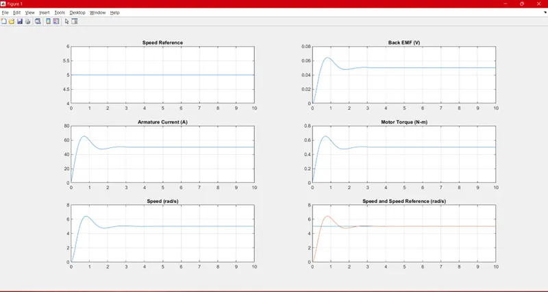
To make best possible result by minimizing the overshoot, undershoot and settling time

Ki = 0.89 (more damped system)

For this value Kp and Kd remain same & changing Ki value for best Result Ki = 16.40

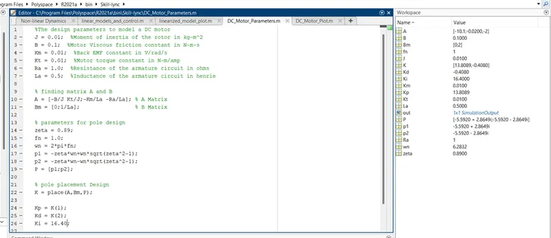
Kp = 13.8089, Kd = -0.4080, Ki = 16.4000

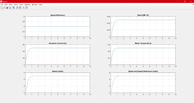
From this we get desired parameters of,

• Settling time < 2 sec
• Overshoot < 5%
• Steady State error < 1%

• 1 rad/s = 9.5493 RPM
• So 5 rad/s = 27 RPM approx

We can minimize for other zeta value also by tunning Kp, Ki, Kd values.

For Example: - zeta = 0.5

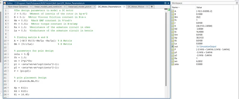
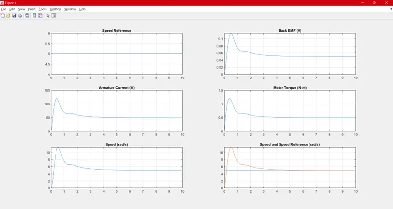
Now taking Kp, Kd, & Ki different value for Over shoot, settling Time and steady state error

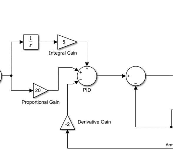
Kp = 20, Ki = 5, Kd = -2

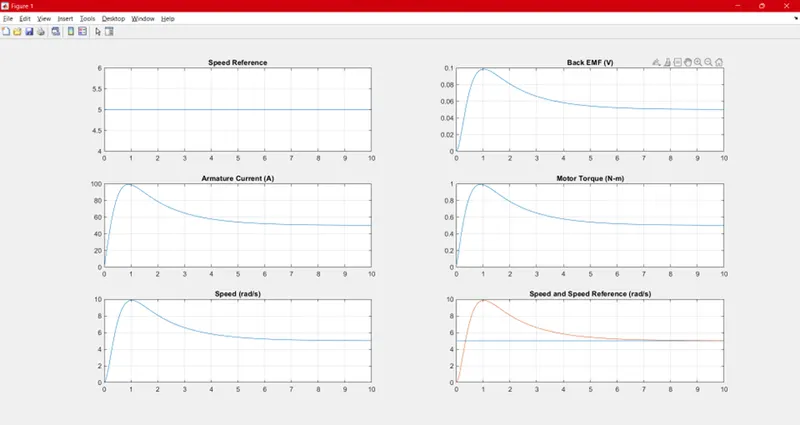
Kp = 0; Ki = 80; KD = 0;

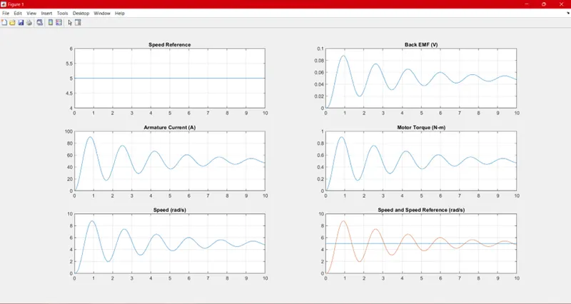
Kp = 20, Kd = -2, Ki = -1

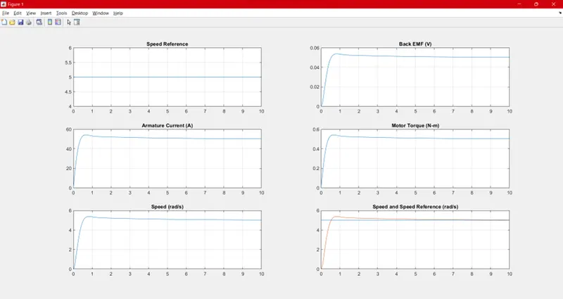
Best response get at

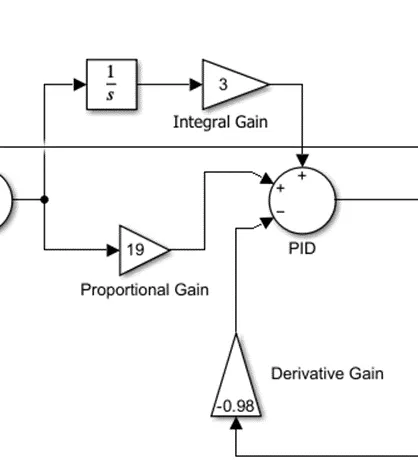
Kp = 19, Kd = -0.98, Ki = 3

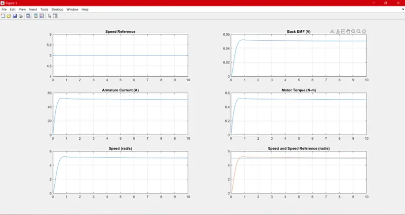
From this we can say that,

• Kp use for increase speed of response
• Kd use for reducing the oscillation
• Ki use for increasing speed with steady state error driven to zero

We can conclude that DC motor working principle and Mathematical modelling from the first principle created in MATLAB script to modelling an Electrical Engineering system. Using MATLAB, we calculated PID values for more damped system (zeta = 0.89) and under damped system (zeta = 0.5). Using this value also created Simulink model with PID gains. Taking Different PID value for stability of a dynamic system.