Project - Speed Control of a Direct Current (DC) motor
The equation is pasted below, which is obtained by means of the kirchoffs law for the Dc motor unit and by means of Newtons law for the load.
The final equation is given below.
w(s)/v(s) = Kt/{(L s+Ra)(Js +B)+Kt*Kb]
The matlab script is given below
%This file contains design paramaters to model a DC motor.
J=0.01; % Moment of inertia of the rotor in kgm^2
B=0.1; % Moment of viscous friction constant in (Nms)
Km=0.01; % Back emf.
Kt=0.01; % Motor Torque
Ra=1.0; % Resistance of aramature circuits(ohm)
La=0.5; % Inductance of aramature circuits(Henries)
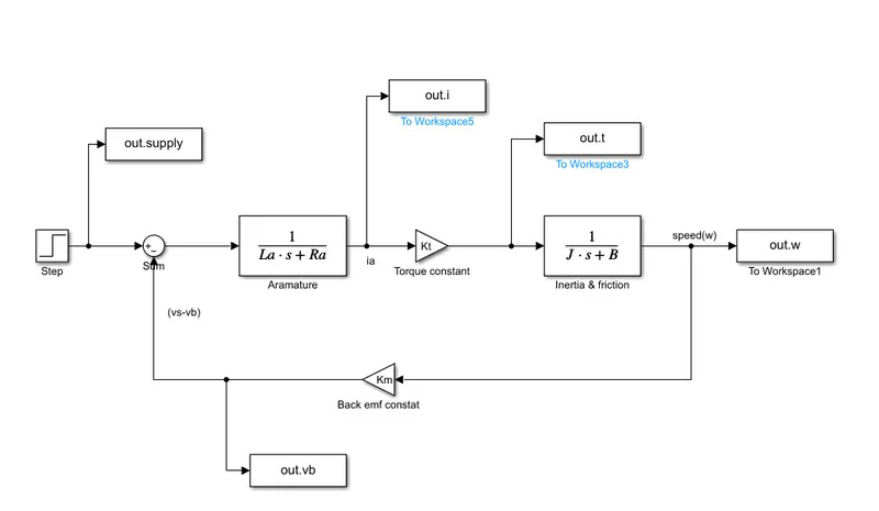
Blocks used
Step Block- To get in the input
Sum Block-To adding the two signals
Clock- To get the times sequence
Workspace- To save the data
Gain Block- To multiply the incoming signal
The simulink model is pasted below.
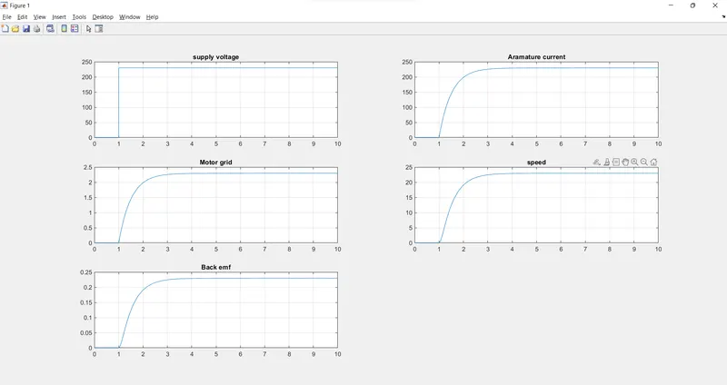
The output has been given below.
By means of the matlab commands the plot are obtained.
The matlab commands are plotting is given below.
>> subplot(321);plot(out.time,out.supply);grid;title('supply voltage');
>> subplot(322);plot(out.time,out.i);grid;title('Aramature current');
>> subplot(323);plot(out.time,out.t);grid;title('Motor grid');
>> subplot(324);plot(out.time,out.w);grid;title('speed');
>> subplot(325);plot(out.time,out.vb);grid;title('Back emf');
>> subplot(322);plot(out.time,out.i);grid;title('Aramature current');
>> subplot(323);plot(out.time,out.t);grid;title('Motor grid');
>> subplot(324);plot(out.time,out.w);grid;title('speed');
>> subplot(325);plot(out.time,out.vb);grid;title('Back emf');
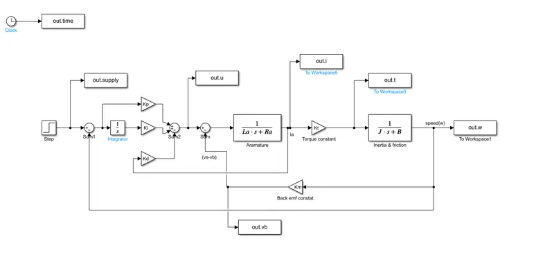
Now the PID controller is implented in order the control the speed of the motor.
The following matrix are obtained by means of the steady state method and the equation for the obaining the matrix are pasted below.
After getting the matrix, the poles are obtained by means of the formula which is given below.
And then then by means of place command the proportional and derivative gain is obained.
The integral gain is kept the 0.0.
The following assumtion are added the matlab script
A=[-B/J Kt/J;-Km/La -Ra/La];
b=[0;1/La];
%%Placement of poles
fn=1;
wn=2*pi*fn;
zeta=0.5;
p1=zeta*wn+wn*sqrt(zeta^2-1);
p2=zeta*wn-wn*sqrt(zeta^2-1);
P=[p1;p2];
k=place(A,b,P);
Kp=K(1); %Proportional gain
Kd=K(2); %Derivative gain
Ki=0.0; %Integative gain
The simulink model after adding the PID controller is given below.
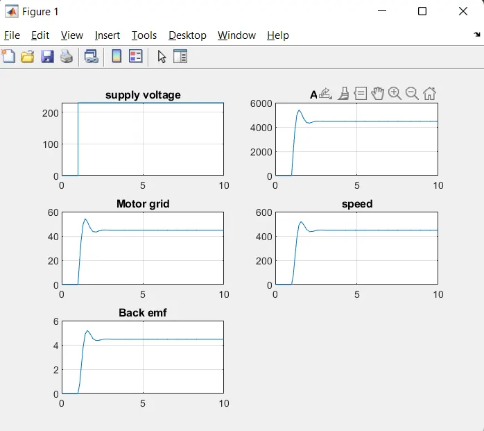
The output by assuming the input voltage as 230 & Ki as 0, is given below.
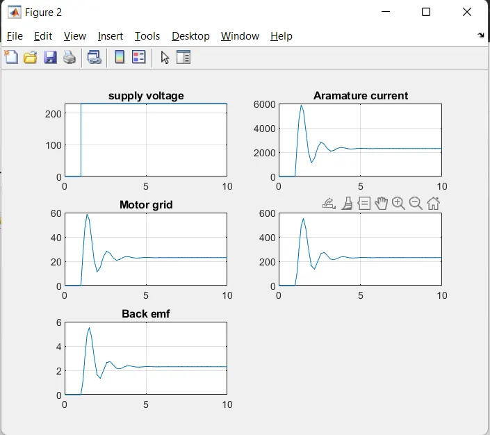
By assuming the Ki as 50,the output is given below.
By assuming the Ki as 30,the output is given below,
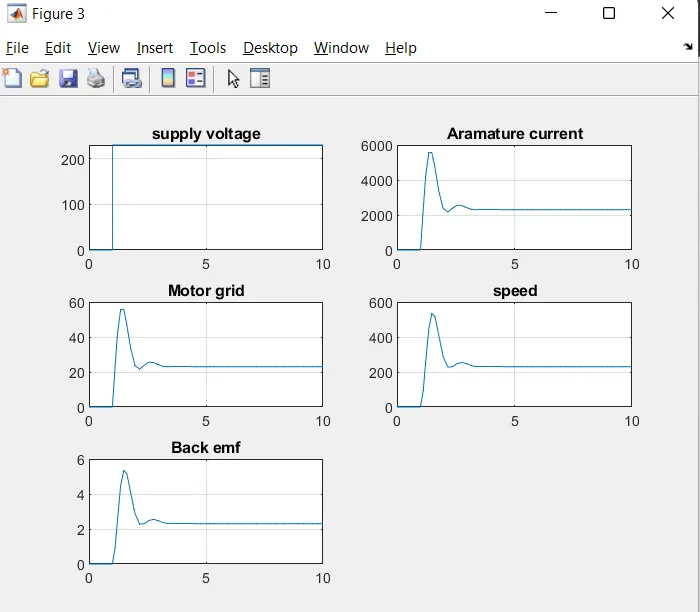
This looks the good design where we have reduced the steady state time, the overshoot & the undershoot.
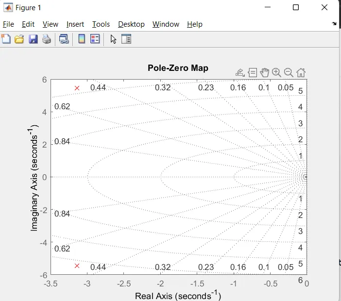
Given transfer function of the poles;
k_dc=1; % the dc gain of the system
s=tf('s');
>> G=k_dc*wn^2/(s^2+2*zeta*wn*s+wn^2);
>> pzmap(G,'r');grid;
>> G=k_dc*wn^2/(s^2+2*zeta*wn*s+wn^2);
>> pzmap(G,'r');grid;