Project 2

Solution:

To modle the development of a forward energy-based fuel consumption model of a P1 hybrid vehicle.

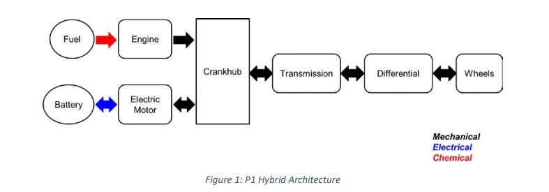
In this model we have both the domains of the Electrical (Motor) and the Mechanical (Engine)are connected in series to the crankshaft, which is why it is called as the P1 Hybrid Vehicle.

We will be using two different sources

• Fuel for engine
• Battery for Electric Motor

This Model is designed by using the Matlab & simulink software

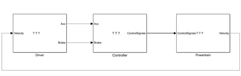
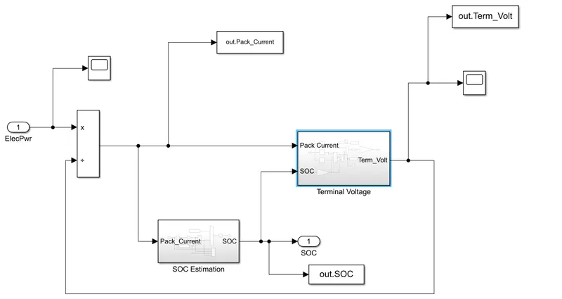
The Model is pasted below.

Main Model

• It consists of 3 different sections which are presented in the above diagram
• The deatailed information is discussed below.

Driver Model

• Input - Velocity ( from the digital meter)
• Output - Brake or Acceralation

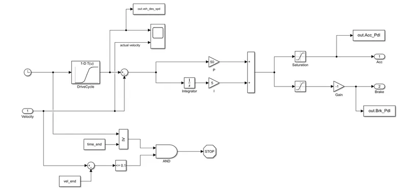
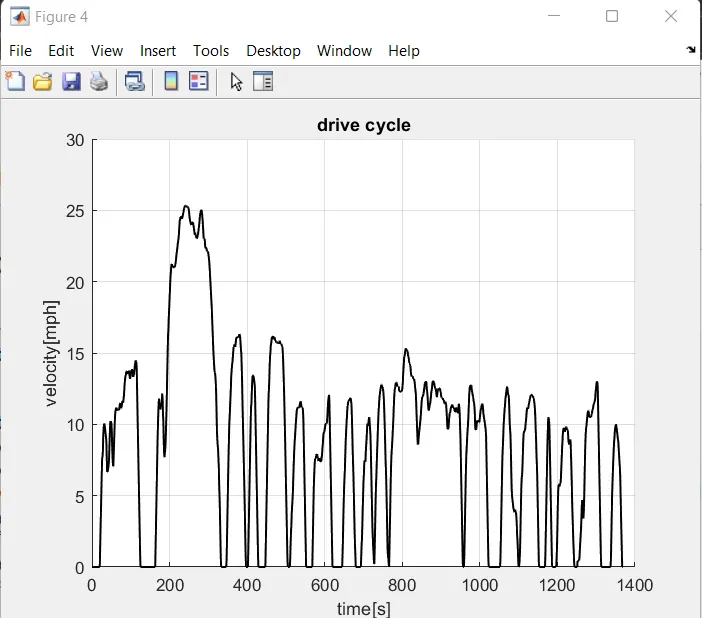
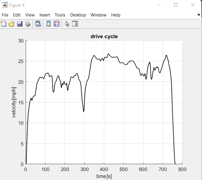
The drive cycle is the various break points of the engine in different road condition depending on the speed and places .

There are various cycles which are mentioned below.

1.Udds

2.Hwfet

3.Ftp

4.Us06

5.Nedc

6.Wltp

The data for the cycles has been provided by which we can modle the P1 hybrid vehicle.

Controller

• The controller is the one of the important section which is used to control the all the systems depending on the drivers requirement.
• It consists of 5 different section which is shown above which is explained in brief below.

Main Controller:

• This is the main controller in which the drivers required is processed by means of applying the following conditions.
• There are four different conditions by which it is used to process the signal
• Condition:1

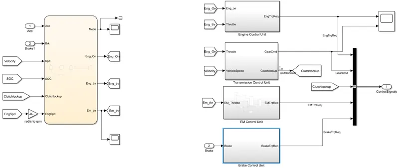
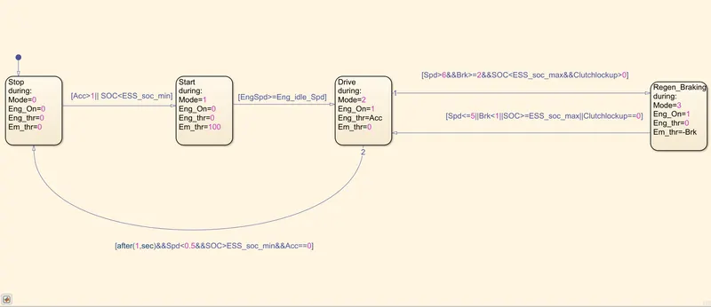
When the vehicle is in the idle, all the systems are in idle and there is no signals flowing

• Condition :2

When the Accleration is pressed by the Driver the Mode 1 is activeted in which it is used to make the Electric motor to switch On

• Condition :3

Now when the speed requiremenet is more than the Engine idle speed which is constat, At this time this mode of 3 gets activated where the Engine gets started

It also consists of one section where the engine is stopped at that time it goes to mode 0 which is the idle conditions

• Condition 4:

In this there are 2 conditions, when the brake is applied the battery is used to charge by means of regenerative braking and the other conditon is nothing but going back to the previous mode as the speed is less.

Engine controller

• Input - Engine_on
• Output - Engine torque required

• From the controller the engine command is used to come here where the engine is used to give the required torque to the crankshaft

Transmission control

• This transmission is used to control the gears by means of the speed and it is used to provide the required torque for the vehicle to move.

Electric Motor controller

• During the start the Electric motor controller is used to control the vehicle to get engine throttle to start as the command from the contrller

Brake control unit

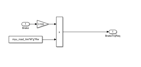
This unit is used to provide the braking which is required for the vehicle to stop

Powertrain

Input - Controller commands

Output - Depending on the controller demand

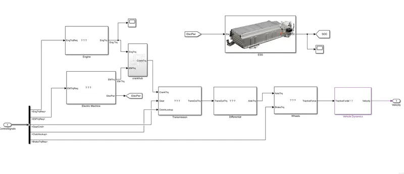
This is the powertrain which is used to provide the Movement to the vehicle based on the controller commands

It consists 8 sections which will be explained below.

Engine

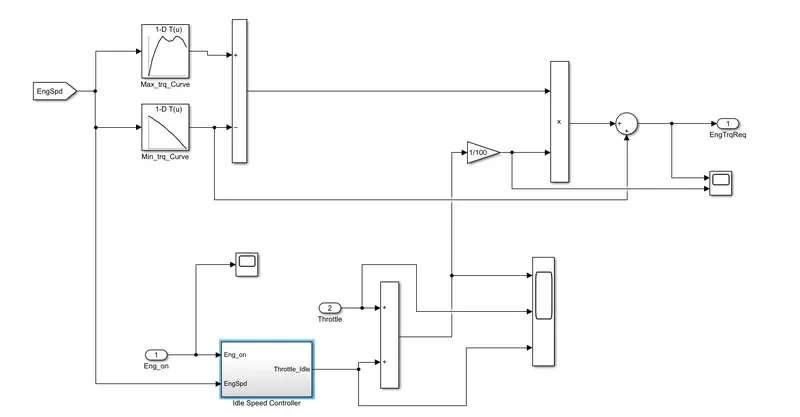
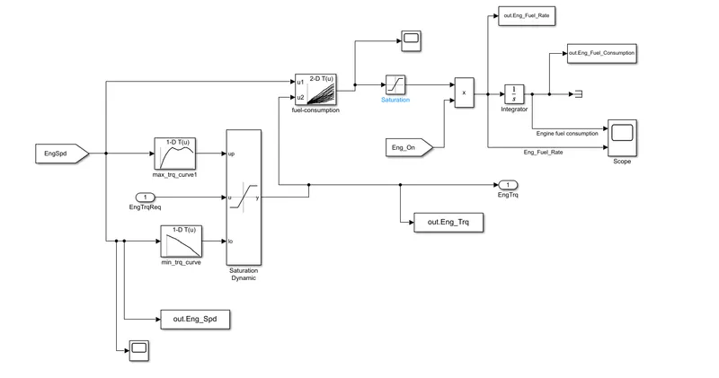
This is engine section where the following data points for the torque requirement and the speed has been obtained from the data given, this is used to give the required data to the crankshaft.

Electric motor

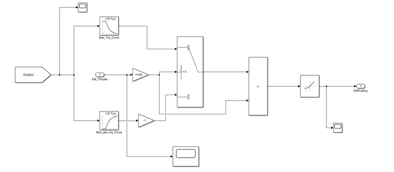
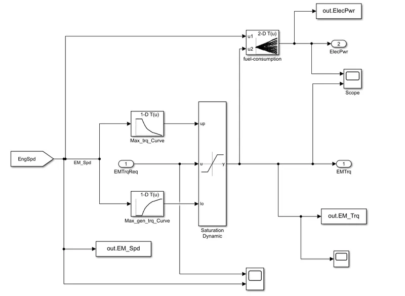
The electric motor is also connected in series where it is used to start the engine and a also used to provide the starting torque which is required for the vehicle for the movement.

Crankshaft

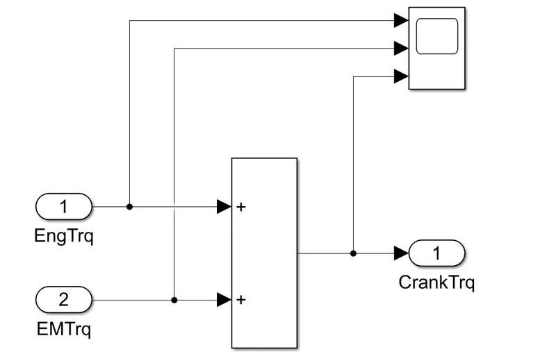
This crankhub consists of crankshaft which is used to get the mechanical movemnt from the engine and also the electric motor.

Transmission

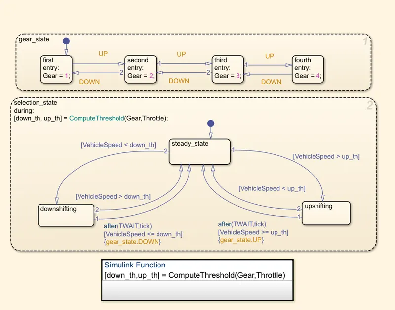
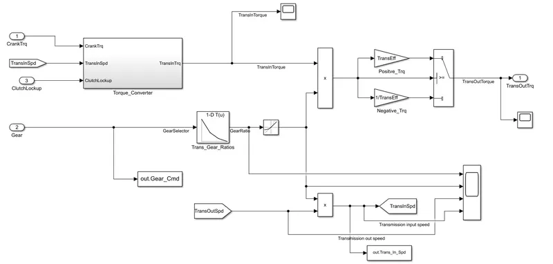
The transmission is used to provide the required for the differential by which the engine power is used efficicently and also the speed is controlled by mean of the various gears.It also consists of lockup clutch where it is used to lockup when it reaches its maximum speed

Differential

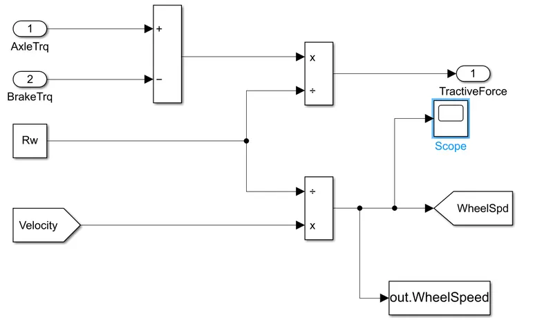
The Differntial is used to transmit the linear motion from the propeller shaft to the wheels

Vehicle Dynamics

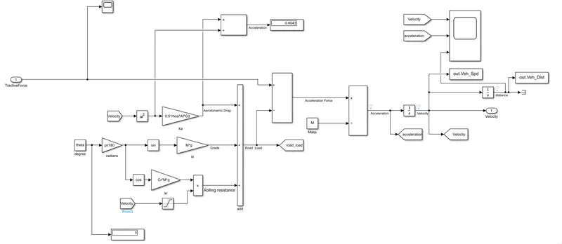
The vehicle dynamics consists of various forces which will be acting on the vehicle while moving , the following forces are mentioned below.

1.Rolling Resistance force

2.Aerodynamics force

3.Acceralation force

4.Grading Force

Battery

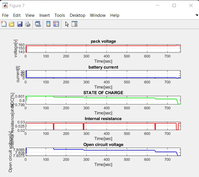
The battery is used to provide the power for the electric motor and also it is used to store the energy while the regenerative braking.And also we can get the Soc from the battery so that we can know the level of charege obtained in the battery.

Matlab Program

The below given program is used to load the various data required for running the simulink model and also for selecting the Drive cycles

The processing program is pasted below which is used for plotting

% file for post-processing the P1 Hybrid vehicle simulation model data

%% Renaming variables

Time = out.tout;

Acc_Pdl = out.Acc_Pdl; % Accelerator pedal [%]

Brk_Pdl = out.Brk_Pdl; % Brake pedal [%]

Gear_Cmd = out.Gear_Cmd; % Transmission gear

Trans_In_Spd = out.Trans_In_Spd*30/pi; % Transmission input speed [rpm]

Trans_Out_Spd = out.Trans_Out_Spd*30/pi;% Transmission output speed [rpm]

Eng_Trq = out.Eng_Trq; % Engine brake torque [Nm]

Eng_Spd = out.Eng_Spd*30/pi; % Engine speed [rpm]

Eng_Fuel_Consump = out.Eng_Fuel_Consumption; % Engine fuel consumption [g]

Eng_Fuel_Rate = out.Eng_Fuel_Rate; %engine fuel rate

Veh_Dist = out.Veh_Dist/1000; % Distance traveled by vehicle [km]

Veh_Spd = out.Veh_Spd*18/5; % Vehicle speed [kmph]

Whl_Spd = out.WheelSpeed*(30/pi); % wheel speed[RPM]

Desired_spd = out.veh_des_spd*(18/5); %desired speed [KMPH]

EM_Spd = out.EM_Spd*30/pi; % E motor speed[rpm]

EM_Trq = out.EM_Trq; % E motor torque[Nm]

EM_Pwr = out.ElecPwr; % E motor input power[W]

V_batt = out.Term_Volt; % battery pack voltage [V]

I_batt = out.Pack_Current; % battery pack current [I]

SOC = out.SOC; % STATE OF CHARGE [%]

RS = out.RS; % internal resistance

VOC = out.VOC; % open circuit voltage

%% Data Analysis

Eng_Pwr = Eng_Spd.*pi/30.*Eng_Trq/1000; % Engine brake power [kW]

rho_petrol = 0.7197; % Density of petrol [kg/L]

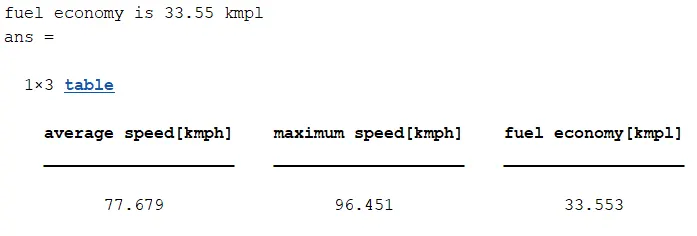
kmpl = Veh_Dist(end)/(Eng_Fuel_Consump(end)/1000/rho_petrol); % Fuel economy [kmpl];

% display fuel Economy of the cycle

formatspec = 'fuel economy is %2.2f kmpl';

fprintf(formatspec,kmpl);

%% Plotting vehicle characteristics time trace

% ploting transmission input,transmission output and wheel speed

figure(1)

hold on

grid on

plot(Time,Trans_In_Spd,'LineWidth',1,'Color','black');

plot(Time,Trans_Out_Spd,'LineWidth',1,'Color','red');

plot(Time,Whl_Spd,'LineWidth',1,'Color','blue');

xlabel('Time[s]')

ylabel('speed[rpm]')

xlim([0,Time(end)]);

legend('trans input','trans Output','wheel speed');

title('transmission input transmission output and wheel speed')

% plotting engine torque,engine power,fuel rate ,fuel consumption

figure(2)

subplot(4,1,1)

hold on

grid on

plot(Time,Eng_Trq,'LineWidth',1,'Color','black');

ylabel('torque[NM]')

xlim([0,Time(end)]);

title('Engine Torque')

subplot(4,1,2)

hold on

grid on

plot(Time,Eng_Pwr,'LineWidth',1,'Color','black');

ylabel('power[KW]')

xlim([0,Time(end)]);

title('Engine Power')

subplot(4,1,3)

hold on

grid on

plot(Time,Eng_Fuel_Rate,'LineWidth',1,'Color','black');

xlim([0,Time(end)]);

xlabel('Time[s]');

ylabel('Engine fuel rate');

title('Engine fuel rate')

subplot(4,1,4)

hold on

grid on

plot(Time,Eng_Fuel_Consump,'LineWidth',1,'Color','black');

xlim([0,Time(end)]);

xlabel('Time[s]');

ylabel('Engine fuel consumption[g]');

title('Engine Fuel Consumption')

% plotting accelerator and brake pedal gear command vehicle desired and actual speed ,vehicle distance

figure(3)

subplot(4,1,1)

hold on

grid on

plot(Time, Acc_Pdl, 'linewidth', 1, 'Color', 'black');

plot(Time, Brk_Pdl, 'linewidth', 1, 'Color', 'red');

ylabel('Pedal [%]')

xlim([0, Time(end)]);

legend('Accel','Brake');

title('Acceleration and brake pedal inputs')

subplot(4,1,2)

hold on

grid on

plot(Time, Gear_Cmd, 'linewidth', 1, 'Color', 'black');

xlim([0, Time(end)]);

xlabel('Time [s]');

ylabel('Gear');

title('gear command')

subplot(4,1,3)

hold on

grid on

plot(Time, Veh_Spd, 'linewidth', 1, 'Color', 'black');

plot(Time, Desired_spd, 'linewidth', 1, 'Color', 'red');

ylabel('Speed [kmph]')

xlim([0, Time(end)]);

legend('actual speed','desired speed');

title('vehicle actual and desired speed')

subplot(4,1,4)

hold on

grid on

plot(Time, Veh_Dist, 'linewidth', 1, 'Color', 'black');

xlim([0, Time(end)]);

xlabel('Time [s]');

ylabel('distance[km]');

title('vehicle distance')

% plotting drive cycle

figure(4)

hold on

grid on

plot(cyc_time,cyc_vel,'LineWidth',1,'Color','black')

xlabel('time[s]')

ylabel('velocity[mph]')

title('drive cycle')

% test result

Avg_speed = sum(Veh_Spd)/length(Veh_Spd);

Max_speed = maxk(Veh_Spd,1);

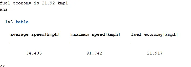
table (Avg_speed,Max_speed,kmpl,'variablenames',{'average speed[kmph]','maximum speed[kmph]','fuel economy[kmpl]'})

%% Plotting engine operating points on engine fuel map

figure('Name','Engine Operating Points');

hold on

grid on

title('Engine Operating Points','fontsize',12);

plot(Eng_map_spd*30/pi,Eng_max_trq,'linewidth',2,'color','r');

p2=line([Eng_map_spd(end)*30/pi Eng_map_spd(end)*30/pi],[0 Eng_max_trq(end)]);

set(p2,'linewidth',1,'linestyle','--','color','k');

p3=line([Eng_map_spd(1)*30/pi Eng_map_spd(1)*30/pi],[0 Eng_max_trq(1)]);

set(p3,'linewidth',1,'linestyle','--','color','k');

[c,h] = contour(Eng_map_spd'*30/pi,Eng_map_trq,Eng_fuel_map');

clabel(c,h);

xlabel('Engine Speed [rpm]');

ylabel('Engine Torque [Nm]');

title('Engine Fuel Consumption Map [g/s]');

legend({'Max Curve','Operating Points'});

axis([Eng_map_spd(1)*30/pi Eng_map_spd(end)*30/pi 0 Eng_map_trq(end)]);

%% Electric Motor

% plotting motor speed ,motor torque,motor input power

figure(6)

subplot(3,1,1)

hold on

grid on

plot(Time,EM_Spd,'LineWidth',1,'Color','b');

ylabel('Speed[rpm]')

xlim([0,Time(end)]);

title('motor speed')

subplot(3,1,2)

hold on

grid on

plot(Time,EM_Trq,'LineWidth',1,'Color','r');

ylabel('torque[Nm]')

xlim([0,Time(end)]);

title('motor torque')

subplot(3,1,3)

hold on

grid on

plot(Time,EM_Pwr,'LineWidth',1,'Color','g');

ylabel('power[W]')

xlim([0,Time(end)]);

title('motor input power')

%% BATTERY

% plotting pack current,voltage,soc,internal resistance,open circuit

% voltage

figure(7)

subplot(5,1,1)

plot(Time,V_batt,'LineWidth',1,'Color','r');

xlabel('Time[sec]');

ylabel('voltage[v]');

title('pack voltage')

xlim([0,Time(end)]);

grid on

subplot(5,1,2)

plot(Time,I_batt,'LineWidth',1,'Color','b');

xlabel('Time[sec]');

ylabel('current[I]');

title('battery current')

xlim([0,Time(end)]);

grid on

subplot(5,1,3)

plot(Time,SOC,'LineWidth',1,'Color','g');

xlabel('Time[sec]');

ylabel('SOC[%]');

title('STATE OF CHARGE')

xlim([0,Time(end)]);

grid on

subplot(5,1,4)

plot(Time,RS,'LineWidth',1,'Color','r');

xlabel('Time[sec]');

ylabel('Internal resistance[ohm]');

title('Internal resistance')

xlim([0,Time(end)]);

grid on

subplot(5,1,5)

plot(Time,VOC,'LineWidth',1,'Color','b');

xlabel('Time[sec]');

ylabel('Open circuit voltage[v]');

title('Open circuit voltage')

xlim([0,Time(end)]);

grid on

%% Plotting engine operating points on engine fuel map

figure('Name','Electric motor Operating Points');

hold on

grid on

title('Electric motor Operating Points','fontsize',12);

p1=plot(EM_map_spd*30/pi,EM_max_trq,'linewidth',2,'color','r');

p4=plot(EM_map_spd*30/pi,EM_max_gen_trq,'LineWidth',2,'Color','b');

p2=line([EM_map_spd(end)*30/pi EM_map_spd(end)*30/pi],[EM_max_gen_trq(end) EM_max_trq(end)]);

set(p2,'linewidth',1,'linestyle','--','color','k');

p3=line([EM_map_spd(1)*30/pi EM_map_spd(1)*30/pi],[EM_max_gen_trq(1) EM_max_gen_trq(1)]);

set(p3,'linewidth',1,'linestyle','--','color','k');

[c,h] = contour(EM_map_spd'*30/pi,EM_map_trq,EM_inpwr_map');

clabel(c,h);

xlabel('Motor Speed [rpm]');

ylabel('motor Torque [Nm]');

title('Motor in power map [W]');

legend([p1 p4 p3],{'Max Curve','regen curve','Operating Points'});

xlim([EM_map_spd(1)*30/pi EM_map_spd(end)*30/pi]);

ylim([EM_max_gen_trq(1) EM_max_trq(1)]);

Post processing Results

1.Drive Cycles

a.Udds

b.Hwfet

2.Fuel Economy Numbers

a.Udds

b.Hwfet

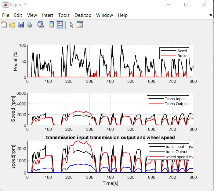
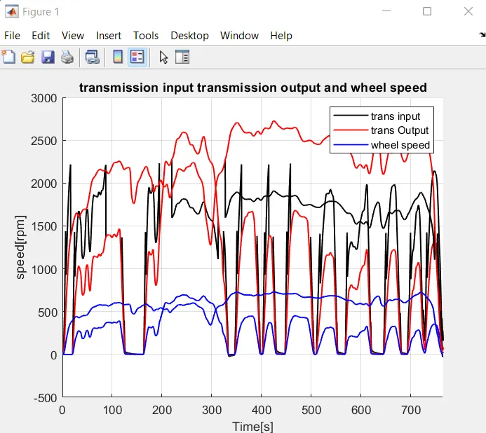
3.Time trace for engine, transmission output and wheel speed

a.Udds

b.Hwfet

• Most of the fluctuatuing input speed is facilated by the torque converter and the transmission input speed fluctuatuing according to the engine torque required to achieve the drive cycle.

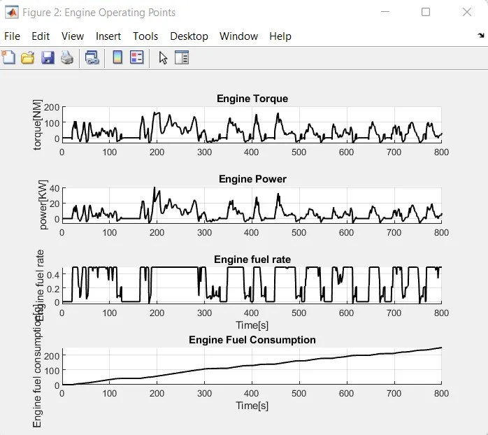
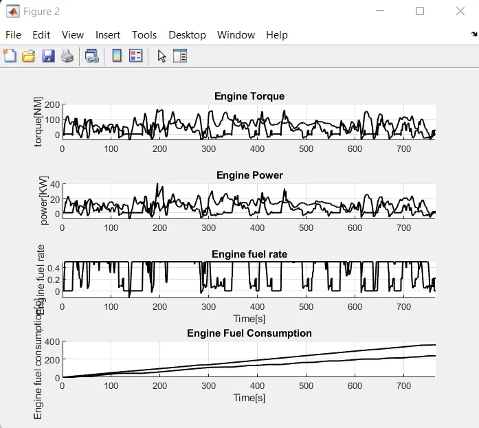
4.Engine torque , engine powerm fuel rate and fuel consumption

a.Udds

b.Hwfet

• The torque requirements of the drive cycles are different and based on that we will be getting the fuel consumption.
• In the highway we will be having the less torque requirement so the fuel econmy is higher in the Hwfer

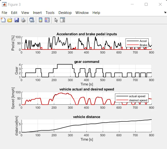
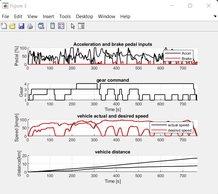
5.Acceletation and brake pedal gear command vehicle desired and actual speed vehicle distance

a.Udds

b.Hwfet

• The acceleration is used a lot by means of the pedal by which we will be getting most of brake torque in the udds
• In highways we will be having the less amount brake as it has also no torque requirement

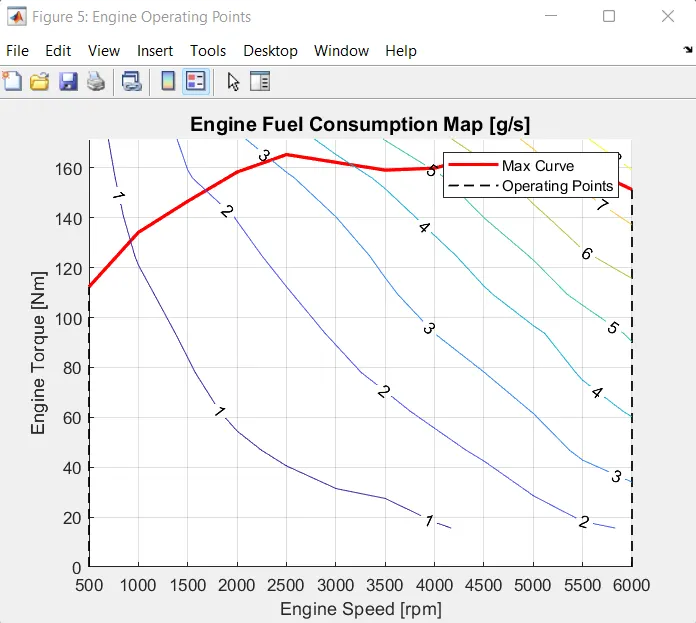
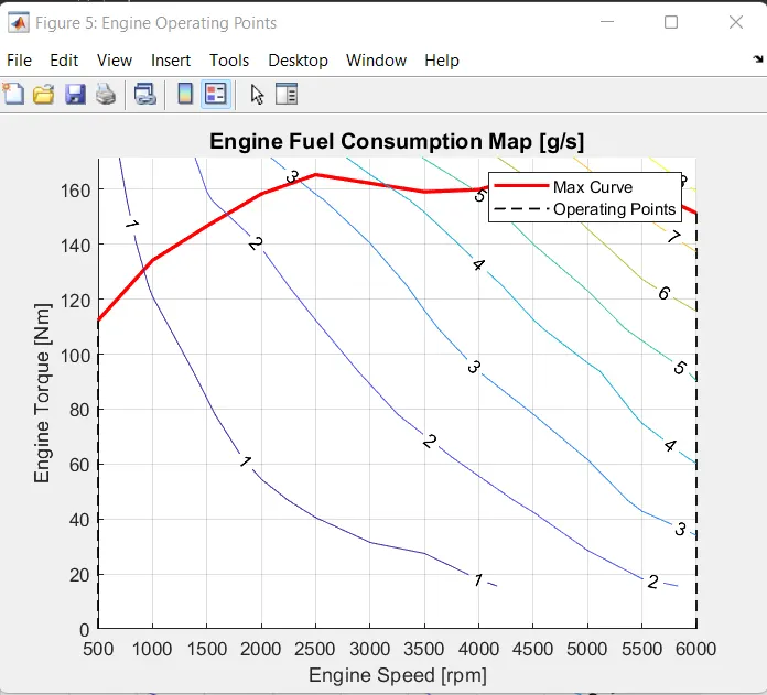
6.Engine operating points on engine fuel map

a.Udds

b.Hwfet

• Both the fuel economy falls depending on the variation of the torque requirement

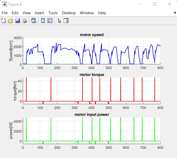
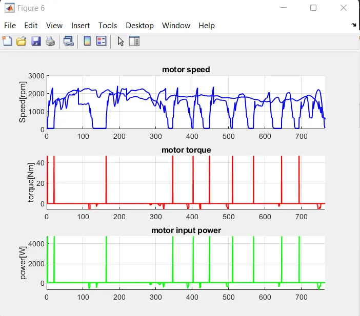
7.Motor speed, torque and motor input power

a.Udds

b.Hwfet

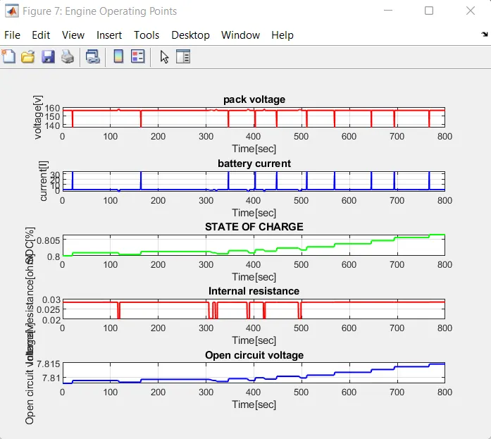
8.The pack voltage, current Soc , voc , Internal resistance

a.Udds

b.Hwfet

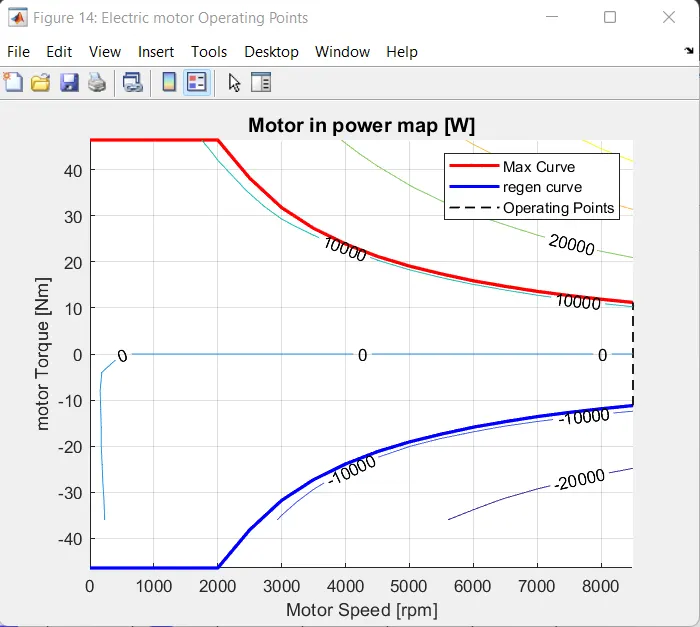
9.The motor Operating points on the motor inputs power map with the motor max motoring and generating torque curves