Project - Speed Control of a Direct Current (DC) motor

Answer:

The given motor shematic diagram doesnt specifically mention whether its an armature controlled or field controled DC motor. So, lets consider the case for an armature controlled DC motor.

Theory:

For an armature controlled DC motor, the field would be kept constant and hence, the field current If woud be constant.

Also we know,

Motor Torque, T = Kt * Ia

Back EMF, Vb = Kb * ω

Now by applying krichoff's voltage law and newton's law in the above schematic

(La * dIa/dt) + (Ra * Ia) = V - (Kb * ω) --------> eqn1

(J * dω/dt) + (B * ω) = (Kt * Ia) --------> eqn2

Y(t) = ω --------> eqn3

We know the general form of state space equation can be represented as:

xdot = Ax + Cu

and

y = Dx + Eu

From eqn1, 2, 3 we can represent the state space equations for DC motor as:

[ωdot Idot] = [-B/J Kt/J ; -Kb/La -Ra/La] * [ω I] + [0 1/La] * V -------> eqn4

Y(t) = [1 0] * [ω I] + [0] * V ------------> eqn5

The laplace transform of eqn1 and eqn2 are:

(La*S*Ia(S)) + (Ra*Ia(S)) = V(S) - (Kb*W(S))

Ia(S) = (V(S) - Kb*W(S)) / (La*S + Ra) -------> eqn6

(J*S*W(S)) + (B*W(S)) = (Kt*Ia(S))

W(S) = (Kt*Ia(S)) / (J*S + B) ---------> eqn7

substituting eqn6 in eqn7

we get the transfer function for the armature controlled DC motor as:

W(S) / V(S) = Kt / [(LaS + Ra)(JS + B) + Kt * Kb] ---------> eqn 8

We know the control signal equation for PID controller is given as:

u(t) = Kp*e(t) + Ki * ∫e(t)dt + Kd * de(t)/dt -----------> eqn9

M-Script:

Below are the assumed design parameters for the DC moor and PID control model:

% Design  parameters to model a DC motor
J = 0.01; % Moment of inertia of the rotor in kg-m^2
B = 0.1; % Motor viscous friction constant in N-m-s
Kb = 0.01; % Back EMF constant in v/rad/s
Kt = 0.01; % Motor torque constant in N-m/amp
Ra = 1.0; % Resistance of the armature circuit in ohms
La = 0.5; % Inductance of the armature circuit in henry

% Design parameters for PID controller
A = [-B/J Kt/J; -Kb/La -Ra/La]; % derived from the state space equations for the DC motor
C = [0; 1/La];

fn = 1; % Natural frequency in Hz
wn = 2*pi*fn; % angular frequency in rad/sec
zeta = 0.9; % damping ratio for under damped case

% Placement of poles
P = roots([1 2*zeta*wn wn^2]); % roots of the denominator polynomial of the transfer function gives the poles
K = place(A,C,P); % Gives the control parameters Kp and Kd

The value for Kp and Kd are determined using the matlab command 'place'

Also the poles where calculated assuming the zeta value as 0.9(under damped case)

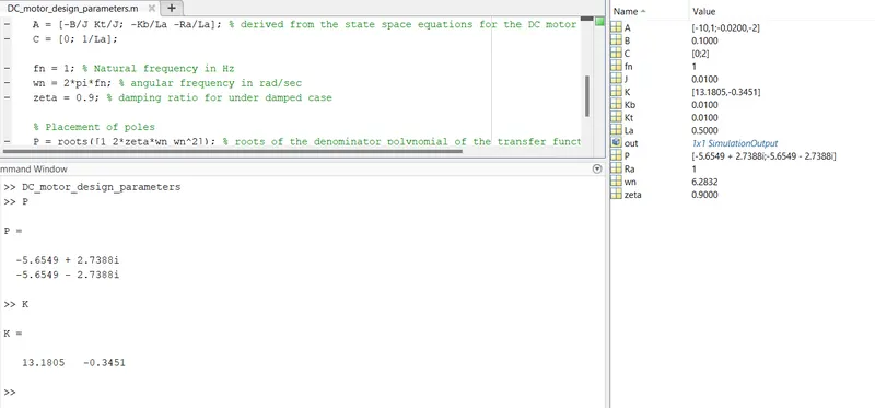
Verified that the poles are in the left plane of s domain and hence system would be stable

Poles = -5.6549 + 2.7388i , -5.6549 - 2.7388i

K = [Kp Kd] = [13.1805 -0.3451]

Ki was determined manually using trial and error method and found that Ki = 32.5 is the optimum value which gave desired output.

Reffering to equations 6, 7, 8 we can first model our DC motor and then the speed control logic using transfer function blocks:

Simulink Model:

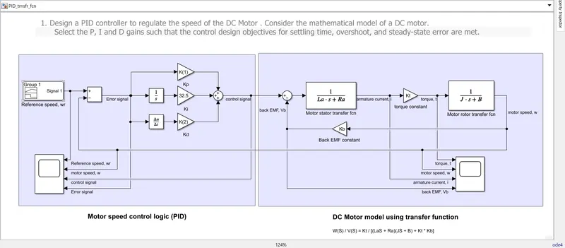
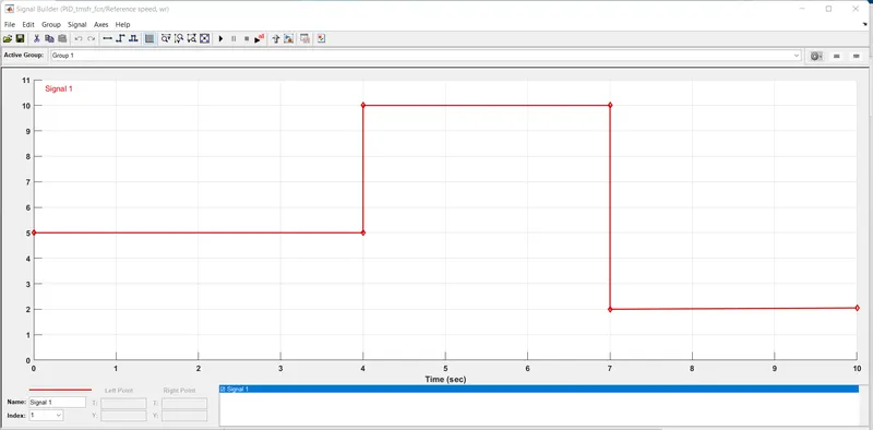
Here we are giving a variying custom step signal as shown below as reference speed, wr.

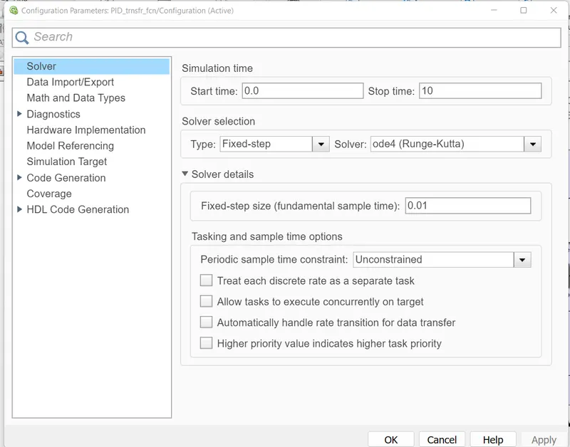
model configuration settings:

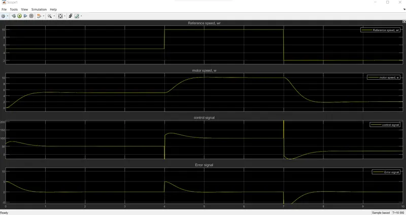
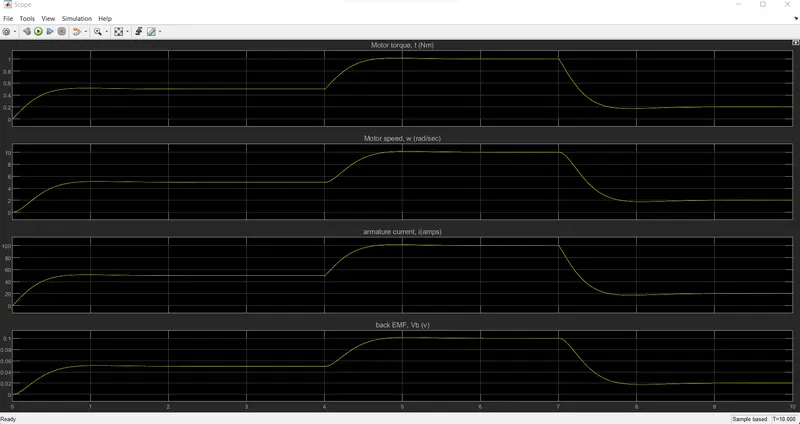
Execution Result:

The simulation was ran for 10 seconds

Conclusion:

Analysing the simulation results, we can state that the actual motor output speed is tracking the reference speed input smooth and fast with,

1. Minimum settling time.

2. Almost no overshoot or undershoot.

3. Zero steady state error.

Hence we can conclude that this is an optimum designed PID controller to regulate the speed of an ideal armature controlled DC motor.