Project - Speed Control of a Direct Current (DC) motor
Schematic diagram of dc motor is shown below:
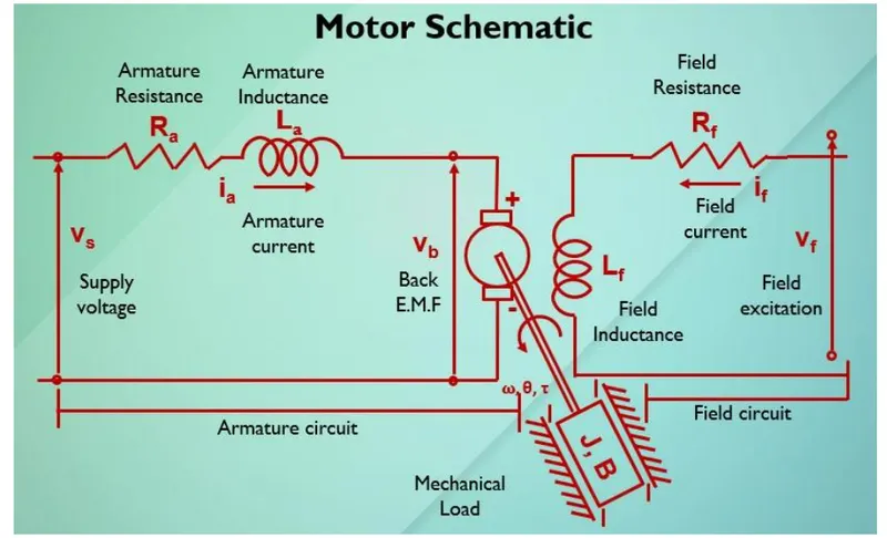
By KVL
Vf = Rf*If + If*(d(If)/dt)
Vs = Rs*Ia + La*(d(Ia)/dt) + Vb
Mathematical Modeling from the first principle and modelling an electrical engineering system equation:
T = Kt*Ia
where Kt is torque constat and Ia is armature current
Vb = Km*w
where Km is back emf constant and w is angular frequency in rad/sec
BY Netwons second law we get
let Kt = Km = K
J*theta_dot + B*theta_dot = K*Ia %Eq1
La*(dIa/dt) + Ra*Ia = K*theta_dot %Eq2
where theta_dot = w (angular Velocity)
Transfer Function
By using laplace transform we get
s(J.s+B)theta(s) = K*Ia(s) %Eq3
(La.s+Ra)Ia(s)= Vs(s)-K.s*theta(s) %Eq4
The final open loop transfer function is
theta_dot(s)/Vs(s) = K/[((J.s+B)(La.s+Ra)+K^2]
MATLAB Script:
% This file contain the design parameters to model DC motor
J = 0.01; % Moment of inertia of rotor in Kg-m^2.
b = 0.1; % Motor Viscous friction constant in N-m_a
Km = 0.01; % Back EMF constant in V/rad/sec
Kt = 0.01; % Motor torque constant in N-m_a.
Ra = 1; % Armature resistance in ohm.
La = 0.5; % Armature inductance in Henery.
%Creating Contineous transfer function.
s = tf('s');
P_motor = Kt/[(J*s+b)*(La*s+Ra)+(Km)^2];
Model:
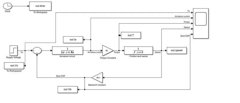
Blocks Used:
Step Block: Here step block is used as supply voltage block which gives the constant supply voltage of 230 volts.
Clock: Clock is used for simulation time
To the Workspace Block: six workspace blocks are used to store the values of simulation time , refrence speed , torque
, armature current , Back emf and speed.
Sum: Sum block is used to perform addition and substraction as per the equation
Transfer function block: Two transfer function block are used
1st transfer function block for armature circuit
2nd transfer function block for friction and inertia system.
Gain Block: two gain blocks are used
1st gain block has gain of Kt
2nd gain block has gain of Km
Scope: Scope blocks are used to get graphical output of the model.
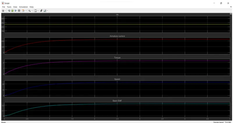
Ploted Graph:
Simulink Model With PID Controller:
PID controller = Kp+(Ki/s)+Kd.s
MATLAB Script as follows:
% This file contain the design parameters to model DC motor
J = 0.01; % Moment of inertia of rotor in Kg-m^2.
b = 0.1; % Motor Viscous friction constant in N-m_a
Km = 0.01; % Back EMF constant in V/rad/sec
Kt = 0.01; % Motor torque constant in N-m_a.
Ra = 1; % Armature resistance in ohm.
La = 0.5; % Armature inductance in Henery.
%Creating Contineous transfer function.
s = tf('s');
P_motor = Kt/[(J*s+b)*(La*s+Ra)+(Km)^2];
% Creating state space model
A = [-b/J Kt/J;-Km/La -Ra/La];
B = [0;1/La];
C = [1 0];
D = 0;
Motor_ss = ss(A,B,C,D);
% Pole placement design parameter
fn=1; % fn=wn/(2*pi), Naturaal frequency in Hz
wn=2*pi*fn; % anugular frequency in rad/sec
zeta=0.5; %Defining Zeta to 0.5
p1=-zeta*wn+wn*sqrt(zeta^2-1); % first pole of charecterastic equation
p2=-zeta*wn-wn*sqrt(zeta^2-1); % second pole of charecterastic equation.
P=[p1;p2]; % P vector stores the two ploes
% Pole placement design using 'place' Command
K=place(A,B,P);
Kp = K(1); % Kp is a proportional gain
Kd = K(2); % Kd is a derivative gain
Ki = 20; % Ki is a integral gain
Model:
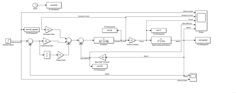
Blocks Used:
Step Block: Here step block is used as refrence speed block which gives the constant refrence speed of 15 rpm.
Clock: Clock is used for simulation time
To the Workspace Block: six workspace blocks are used to store the values of simulation time , refrence speed , torque
, armature current , Back emf and speed.
Sum: Sum block is used to perform addition and substraction as per the equation
Transfer function block: Two transfer function block are used
1st transfer function block for armature circuit
2nd transfer function block for friction and inertia system.
Gain Block: Five gain blocks are used
1st gain block has gain of Kp
2nd gain block has gain of Kd
3rd gain block has gain of Ki
4th gain block has gain of Kt
5th gain block has gain of Km
Scope: Scope blocks are used to get graphical output of the model.
Outputs:
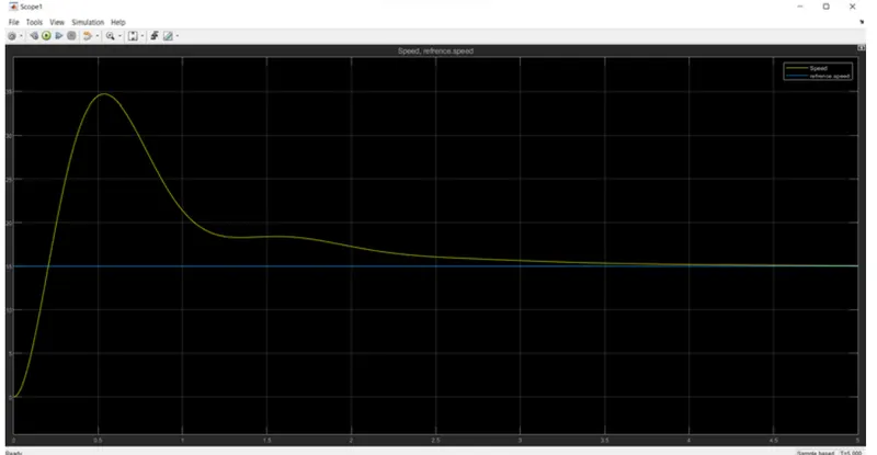
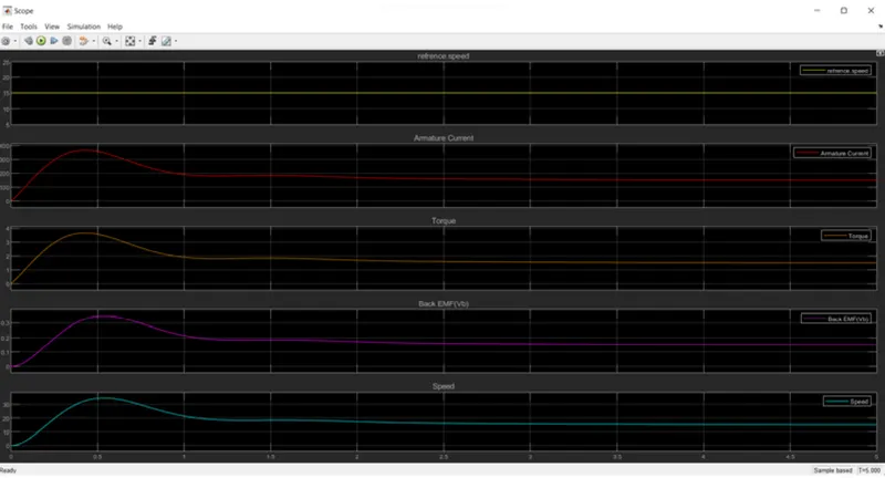
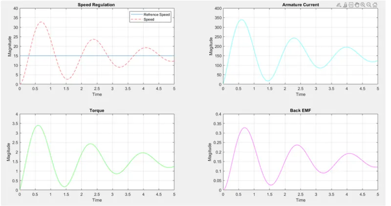
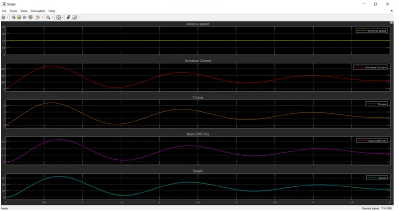
The system is considered for zeta = 0.5.
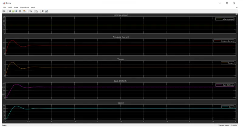
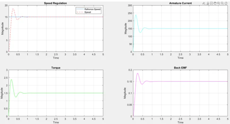
For standered values means using zeta we get Kp,Kd values 38.3133, -2.8584 respectively and Ki considered as 20.
For the above values the result is as follows
Scope output:
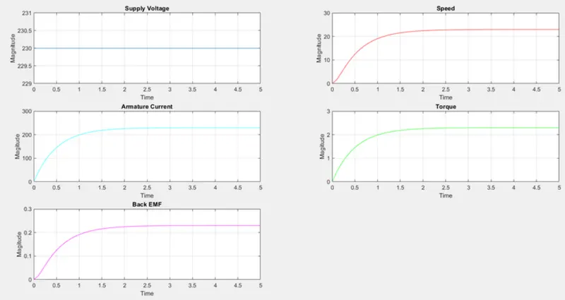
PLOTS :- We use the following script to plot the plots
% plotting the outputs
subplot 321
plot(out.time,out.Vs); % plotting time Vs supply voltage plot in solid blue line
grid;
Z=[0 5 229 231]; axis(Z);
% Labeling the plots
xlabel('Time'); ylabel('Magnitude');title('Supply Voltage');
subplot 322
% plotting time Vs speed plot in red line
plot(out.time,out.speed,'r');
% Labeling the plots
xlabel('Time');ylabel('Magnitude');title('Speed');
grid
% setting the axis
T=[0 5 0 30];axis(T);
subplot 323
plot(out.time,out.Ia,'c')
% labelling the plots
xlabel('Time');ylabel('Magitude');title('Armature Current');
grid;
% setting the axis
V=[0 5 0 300];axis(V);
subplot 324
plot(out.time,out.T,'g')
% labelling the plots
xlabel('Time');ylabel('Magitude');title('Torque');
grid;
W=[0 5 0 3];axis(W);
subplot 325
plot(out.time,out.Vb,'m')
% labelling the plots
xlabel('Time');ylabel('Magitude');title('Back EMF');
grid;
X=[0 5 0 0.3];axis(X);
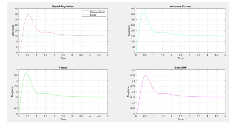
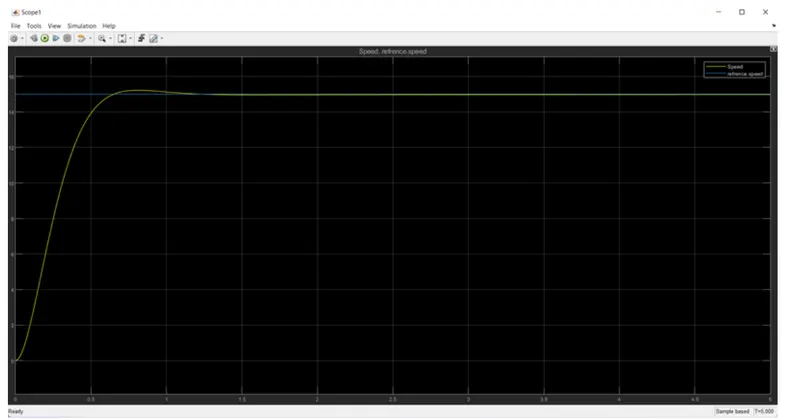
To make the best performance we get by minimizing the overshoot and less settling time.
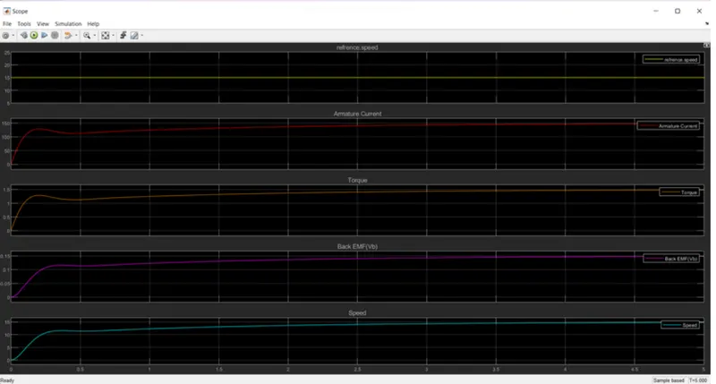
For Example by tunning the gains for one set of values Kp = 20, Kd = -0.92, Ki = 3;
WE got
1) settling time < 2 Sec.
2) overshoot < 5%
3) steady state error < 1%
Scope output:
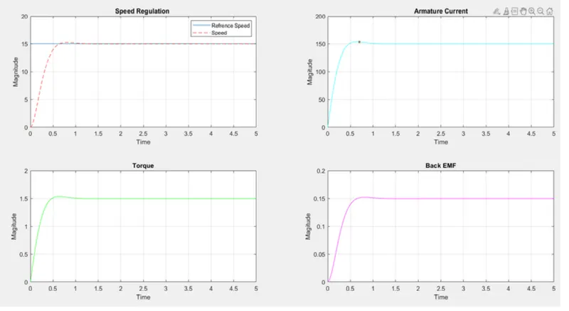
We can minimize more and we can increase the overshoot,settling time and steady state error by tunning Kp,Ki Kd
values the response as follows:
1) Use Kp to increase the speed of response.
2) Use of Kd to reduce oscillations
3) Use Ki to increase the speed with which the steady state error is driven to zero
For example:
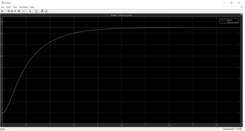
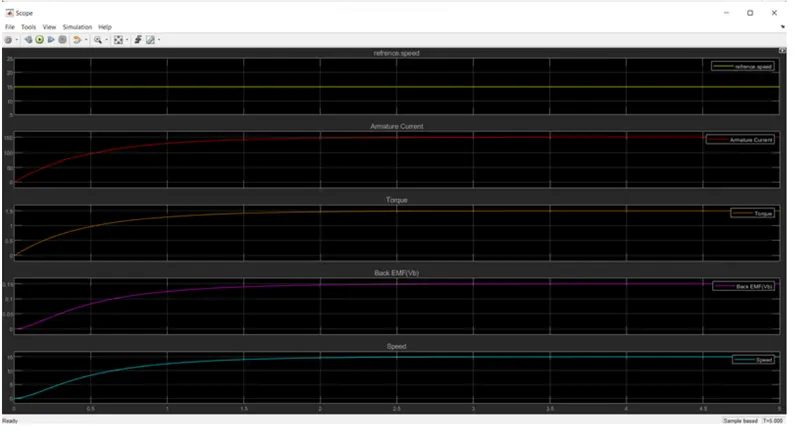
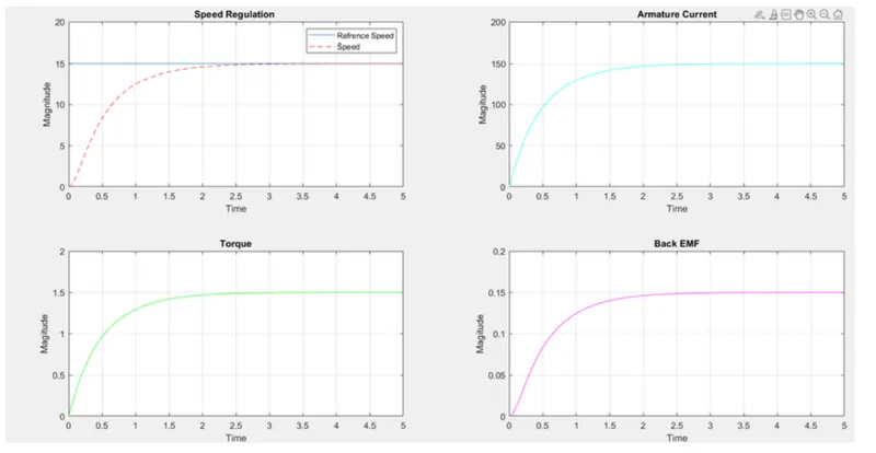
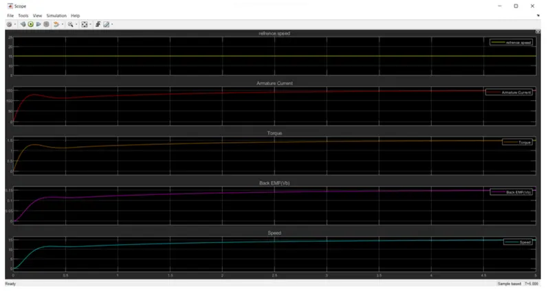
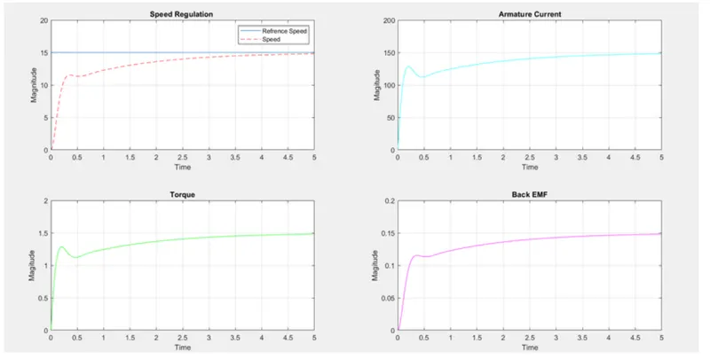
Case - 1
for Kp = 10 ; Ki = 50 ; Kd = 2
Case - 2
for Kp = 50 ; Ki = 50 ; Kd = 2 ;
scope:
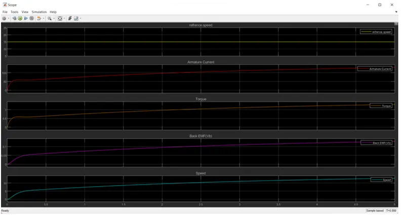
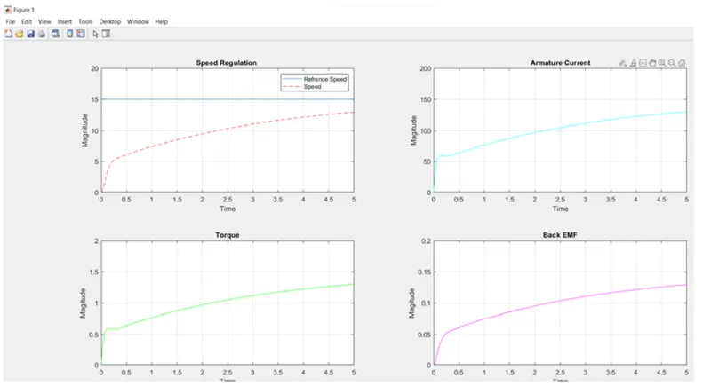
Case - 3
for Kp = 50 ; Ki = 50 ; Kd = 10 ;
scope:
Case - 4
for Kp = 20 ; Ki = 50 ; Kd = -2 ;
scope:
Case - 5
for Kp = 100 ; Ki = 300 ; Kd = 1 ;
scope: