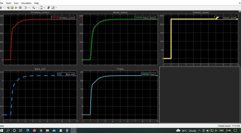
Project - Speed Control of a Direct Current (DC) motor

In this project to design the Proportional, Integral, and Derivative (PID) control design knowledge gained in the training to design, develop and test a controller to maintain a desired speed for the motor.

Key Highlights:

• Mathematical modeling from the first principles
• Modeling an Electrical Engineering system
• Simulink based modeling
• Control law design and test
• Stability of a dynamic system
• Mathematical modeling from the first principles

The Speed control of a DC motor is either done manually by the operator or by means of an automatic control device.This is different to speed regulation where the speed is trying to be maintained or regulated against the natural change in speed due to a change in the load on the shaft so the speed can be varied by changing:

• 1. The terminal voltage of the armature V
  2. The external resistance in armature circuit R_a
  3. The flux per pole

• Terminal voltage and external resistance involve a change that affects the armature circuit while flux involves a change in the maginetic field . Therefore speed control of DC motor can be classified into:

  1. Armature Control Methods
  2. Field Control Methods

Simulink model :

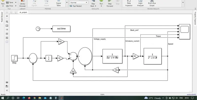
• Here first we need to creat simulink model of the DC motor and make it as subsytem called the DC motor
• So next the subsytem of DC motor is connected to the discrete PID controller which helps in maintaining the desired speed
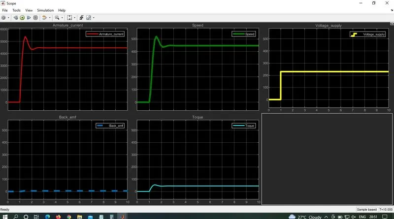
• So after the PID controller we need to start with the kp ki kd such as 1.0 1.0 0 after tunin accordingly so by this we can adjust the kp ki kd values as 31.5 82.3 2.3
• Which is used to obtaine the control design objectives

Parameters:

J=0.01; % moment of inertia

B=0.1; % motor viscous friction

Km=0.01;% Back Emf

Kt=0.01; % Motor Torque Constant

Ra=1; % Armature Resistance

La=0.5;%Armature Inductance

M-script

J=0.01
B=0.1
Kb=0.01
Kt=0.01
Ra=1.0
La=0.5
Ki=0.0001
A=[-B/J Kt/J; -Km/La -Ra/La];
B1=[0 ; 1/La];
zeta = 0.5;
wn=6.28;
p1 = -zeta*wn+wn*sqrt(zeta^2-1);
p2= -zeta*wn-wn*sqrt(zeta^2-1);
P = [p1;p2]
K = place(A,B1,P)
Kp=K(1)
Kd=K(2)

MODEL

SCOPE

AFTER

Kp=31.58

Ki=82.37
Kd=2.35

m-script

J=0.01
B=0.1
Kb=0.01
Kt=0.01
Ra=1.0
La=0.5
Ki=82.37
A=[-B/J Kt/J; -Km/La -Ra/La];
B1=[0 ; 1/La];
zeta = 0.5;
wn=6.28;
p1 = -zeta*wn+wn*sqrt(zeta^2-1);
p2= -zeta*wn-wn*sqrt(zeta^2-1);
P = [p1;p2]
K = place(A,B1,P)
Kp=31.58
Kd=2.35