Project - Speed Control of a Direct Current (DC) motor

Project – Speed control of a DC Motor

Aim: To design a PID controller for the speed control of a DC Motor

Objective: In this project, a Simulink model for the DC motor will be first developed per the schematic shown in Figure 1.

Use the Proportional, Integral, and Derivative (PID) control design knowledge gained in the training to design, develop and test a controller to maintain a desired speed for the motor.

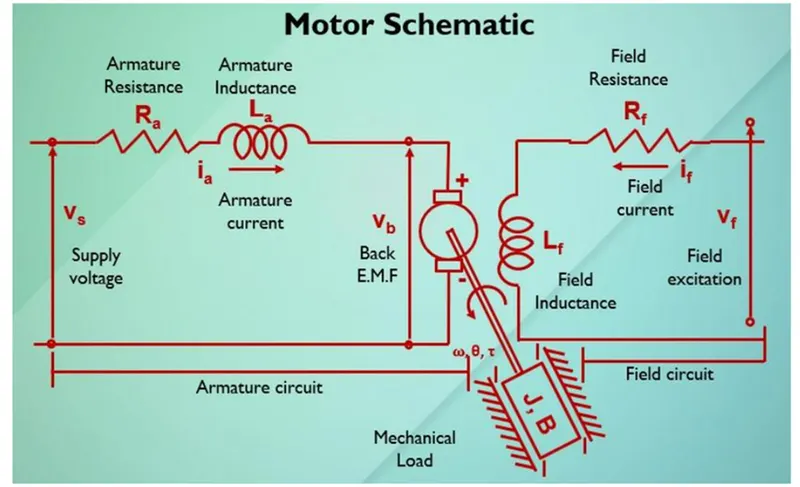
Solution:

In this project, we have been tasked with designing a PID controller for the speed control of a DC motor. DC motors have speed-control capability, which means that speed, torque and even direction of rotation can be changed at any time to meet new conditions. PID controllers are commonly used to regulate the time-domain behaviour of many different types of dynamic plants. These controllers are extremely popular because they can usually provide good closed-loop response characteristics, can be tuned using relatively simple design rules, and are easy to construct using either analog or digital components. Consider the feedback system architecture that is shown in Fig. 1 where it can be assumed that the plant is a DC motor whose speed must be accurately regulated.

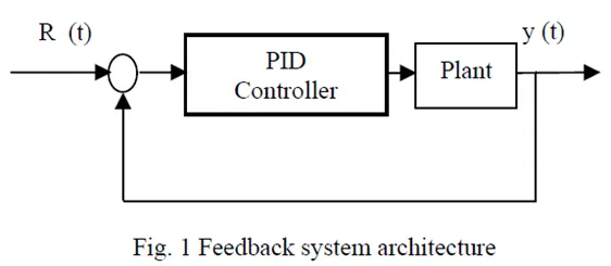
The PID controller is placed in the forward path, so that its output becomes the voltage applied to the motor's armature. The feedback signal is a velocity, measured by a tachometer. The output velocity signal y (t) is summed with a reference or command signal R (t) to form the error signal e (t). Finally, the error signal is the input to the PID controller. The PID controller is defined by the following relationship between the controller input e (t) and the controller output u (t) that is applied to the motor armature:

The electric circuit of the armature and the free body diagram of the rotor are shown below:

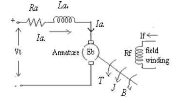
where, R_a=Armature Resistance,

L_a=Armature self inductance caused by armature flux,

i_a= Armature current,

i_f= field current,

E_b=Back EMF in armature,

V_s =Applied voltage,

T=Torque developed by the motor,

θ = Angular displacement of the motor shaft,

Ј =Equivalent moment of inertia of motor shaft & load referred to the motor,

B= Equivalent Coefficient of friction of motor shaft & load referred to the motor.

Applying Kirchoff’s voltage law to the circuit,

V_s = R_a * i_a + L_a * di_a / dt + V_b ……….. (1)

Also, E_b = K_b * dθ/dt ………….. (2)

We know the torque and armature current equation to be,

T = K_t * i_a ………….. (3)

where, K_b = back emf constant

K_t = torque constant

Also, torque is given by,

T = J*d²θ/dt² + B * dθ/dt² ………(4)

Taking the Laplace transform of the above equations,

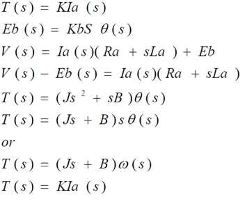
The transfer function based on the above transform can be given as:

For building the Simulink models, I have taken into consideration the transfer functions as well as the differential equations and have built two models accordingly. The control here is for the output speed of the motor and the same has been set at 2000 rpm. The Simulink models for the two approaches are as follows:

Simulink model link:

https://drive.google.com/drive/folders/1ufzRo9FTWbBs5soOYt53dViZKMewvJEE?usp=sharing

1) Transfer function based model:

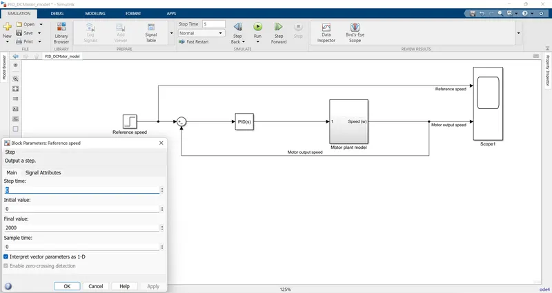
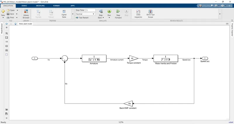
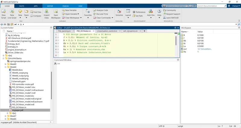
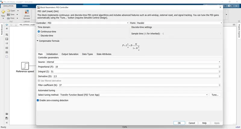
The PID gains have been determined by trial and error method. The use of the tuner app in the PID block itself helps us have an idea about the probable values of the gain. The gains have been accordingly set as:

Output:

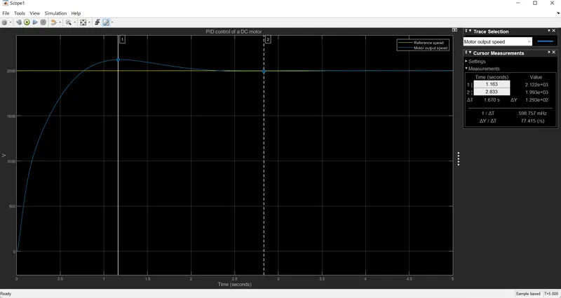
As can be seen, the motor output speed sets off from point 0 as the reference is set at 2000 rpm. In a bid to chase and achieve the reference speed, the motor overshoots (line 1) about a 120 units but then reverses and follows the reference again. In its attempt to stabilise it undershoots (line 2) slightly and then finally stabilises at about 3.5 seconds. Thus our controller helps us control the output speed of the DC motor with respect to the reference speed.

2) Differential equation based model:

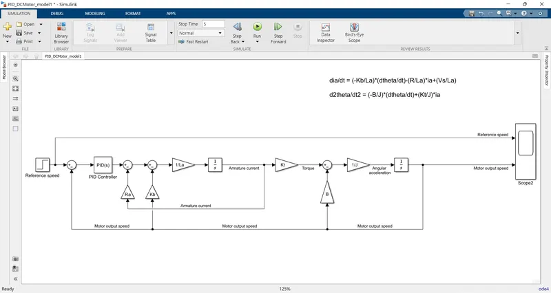
This model is built from the differential equations without transforming them into the Laplace domain. The output results should be inline with the above results to ascertain the correctness of the model.

Output:

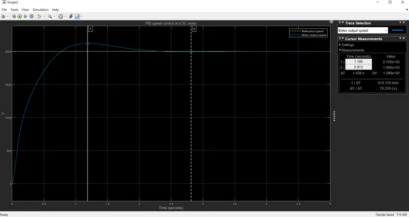
As can be seen the output is in close proximity to the above results. Hence, this model has also been able to meet our required objective of the output speed control of the DC motor.

References:

MATLAB documentation

!!!Thank You!!!