Challenge Week 4 - Curve Fitting

Challenge on Curve Fitting

Aim: To write a program in Matlab for fitting curves of different degrees of polynomials to a given set of raw data

The data for the same is:

Objectives:

1) To write a code to fit a linear and cubic polynomial for the data. Also, for the split wise method.

2) Plot these curves along with raw data points.

3) Explaining the parameters used to measure the fitness the characteristics of the curves.

What is Curve Fitting?

Before getting started with the code, let’s get an understanding of the subject first. So, curve fitting is a process of constructing a curve or mathematical function which possesses the closest proximity to the real series of data. By curve fitting we can mathematically construct the functional relationship between the observed dataset and parameter values. It is highly effective in mathematical modelling of some natural processes. Let’s get to know more of it in depth.

For root finding, we used a given function f(x) to identify where it crossed zero i.e where does f(x)=0? However, where does this given function come from in the first place? Well, the answer to it is:

• Analytical models of phenomena (e.g. equations from physics) or,
• On creating an equation from observed data

Well, the second pointer is what we will be actually making use of for curve fitting. For that, we will first begin with a linear function and go on increasing the polynomial degree to find a good fit. Now, let’s know about how to find that.

Linear curve fitting (linear regression)

Given the general form of a straight line

f(x)= ax+b,

i) How can we pick the coefficients that best fits the line to the data?

ii) What makes a particular straight line a ‘good’ fit?

iii) Why does the blue line appear to us to fit the trend better?

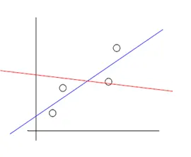
For it we need to taken into account some considerations, which are,

• Consider the distance between the data and points on the line
• Add up the length of all the red and blue vertical lines
• This is an expression of the ‘error’ between data and fitted line
• The one line that provides a minimum error is then the ‘best’ straight line

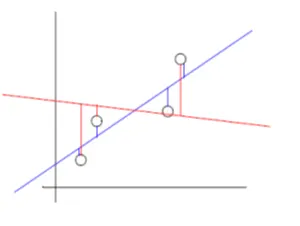
Quantifying errors in a curve fit

Assumptions:

1) Positive or negative errors have the same value (data point is above or below the line)

2) Weight greater errors more heavily

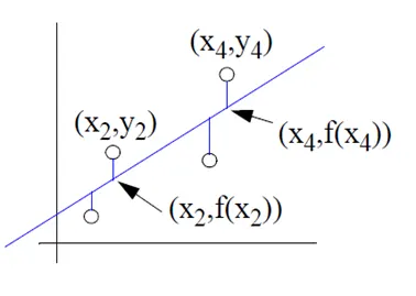
Well, to achieve this, all we need to do is square the errors. So, let’s denote data values as (x, y) and points on the fitted line as (x, f(x))

err = ∑ (d_i)² = (y1-f(x1))² + (y2-f(x2))² + (y3-f(x3))² + (y4-f(x4))²

Our fit is a straight line, so lets substitute f(x)= ax+b

The best-fit line has the least error between the line and data points. The above method is called the least squares approach, since we minimize the squares of the error. All we have to do now is to calculate the values of the coefficients ‘a’ and ‘b’ to derive a function. And how do we do that? Well, we need to recall our calculus classes for it. So, how do we find the minimum of a given function? For it:

• The derivative describes the slope
• Equating the slope to zero gives us the minimum

Now, taking the derivatives of the error with respect to a and b and equating the same to zero,

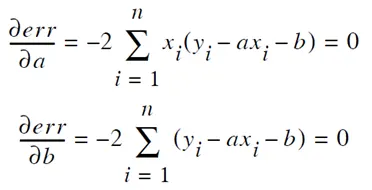
Solving for a and b,

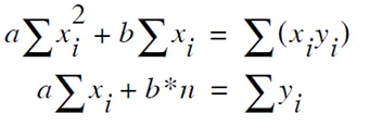
Putting it into a matrix,

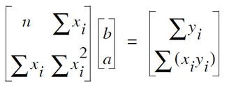
The unknowns here are just a and b. So how do we solve it? Worry not; Gauss-elimination is there at our rescue. How does it work, though?

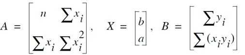
So accordingly,

AX = B

We can get the values for matrix X by,

X = A^-1 B where, A^-1 is the inverse of A.

That’s it. On obtaining the coefficients, we have a best-fit function that has the closest proximity to our given set of data.

Higher order polynomials

We started the linear curve fit by choosing a generic form of the straight-line f(x) = ax + b. This is just one kind of function. There are an infinite number of generic forms we could choose from, for almost any shape we want. Consider the general form of a polynomial of order j

Just as we did for the linear curve fitting, we need to follow all the procedures and get the values of all the coefficients.

But, how do we know whether our curve is a best fit or not? Well, that is governed by some parameters. Let’s get to know them.

Evaluating Goodness of Fit

Goodness-of-Fit Statistics

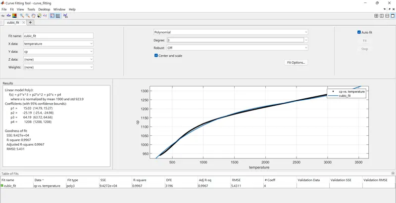
After using graphical methods to evaluate the goodness of fit, you should examine the goodness-of-fit statistics. Curve Fitting Toolbox™ software supports these goodness-of-fit statistics for parametric models:

• The sum of squares due to error (SSE)
• R-square
• Adjusted R-square
• Root mean squared error (RMSE).

Sum of Squares Due to Error (SSE)

This statistic measures the total deviation of the response values from the fit to the response values. It is also called the summed square of residuals and is usually labelled as SSE.

SSE=`sum_(i=1)^n`(y_i-f(x_i))²

A value closer to 0 indicates that the model has a smaller random error component, and that the fit will be more useful for prediction.

R-Square

This statistic measures how successful the fit is in explaining the variation of the data. Put another way, R-square is the square of the correlation between the response values and the predicted response values. It is also called the square of the multiple correlation coefficient and the coefficient of multiple determination.

R-square is defined as the ratio of the sum of squares of the regression (SSR) and the total sum of squares (SST). SSR is defined as

SSR=`sum_(i=1)^n`(y_i-mean)²

SSR is also called the sum of squares about the mean

Also, SST = SSR + SSE

Given these definitions, R-square is expressed as

R-square=SSR/SST

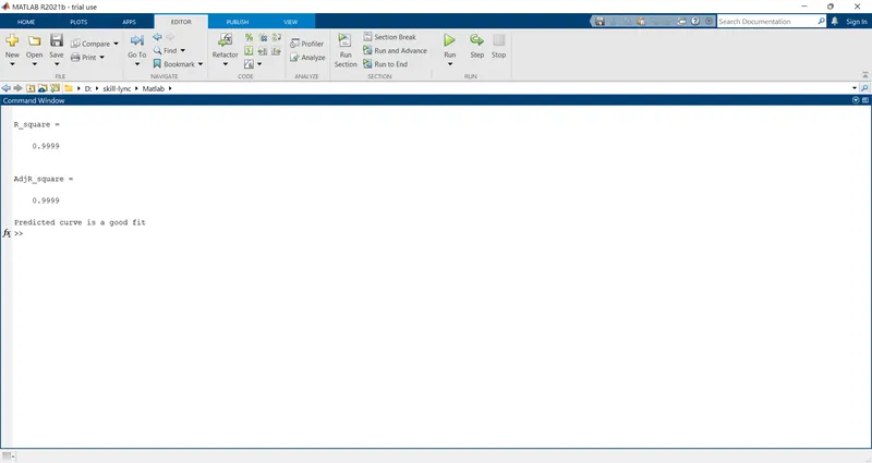
R-square can take any value between 0 and 1, with a value closer to 1 indicating that a greater proportion of variance is accounted for by the model. For example, an R-square value of 0.8234 means that the fit explains 82.34% of the total variation in the data about the average. Typically, a value or R-square greater than 0.95 quantifies the curve as a best fit whereas a value of 1 deems it to be a perfect fit.

If you increase the number of fitted coefficients in your model, R-square will increase although the fit may not improve in a practical sense. To avoid this situation, you should use the degrees of freedom adjusted R-square statistic described below.

Note that it is possible to get a negative R-square for equations that do not contain a constant term. Because R-square is defined as the proportion of variance explained by the fit, if the fit is actually worse than just fitting a horizontal line then R-square is negative. In this case, R-square cannot be interpreted as the square of a correlation. Such situations indicate that a constant term should be added to the model.

Degrees of Freedom Adjusted R-Square

This statistic uses the R-square statistic defined above, and adjusts it based on the residual degrees of freedom. The residual degrees of freedom is defined as the number of response values n minus the number of fitted coefficients m estimated from the response values.

v = n – m

v indicates the number of independent pieces of information involving the n data points that are required to calculate the sum of squares. Note that if parameters are bounded and one or more of the estimates are at their bounds, then those estimates are regarded as fixed. The degrees of freedom is increased by the number of such parameters.

The adjusted R-square statistic is generally the best indicator of the fit quality when you compare two models that are nested — that is, a series of models each of which adds additional coefficients to the previous model.

Adjusted R-square= 1−[(R-square*(n−1))/n-v-1]

The adjusted R-square statistic can take on any value less than or equal to 1, with a value closer to 1 indicating a better fit. Negative values can occur when the model contains terms that do not help to predict the response.

Root Mean Squared Error

This statistic is also known as the fit standard error and the standard error of the regression. It is an estimate of the standard deviation of the random component in the data, and is defined as

RMSE=`sqrt ((SSE)/n)` where, n= total number of data points available

Just as with SSE, an RMSE value closer to 0 indicates a fit that is more useful for prediction.

Understanding the code

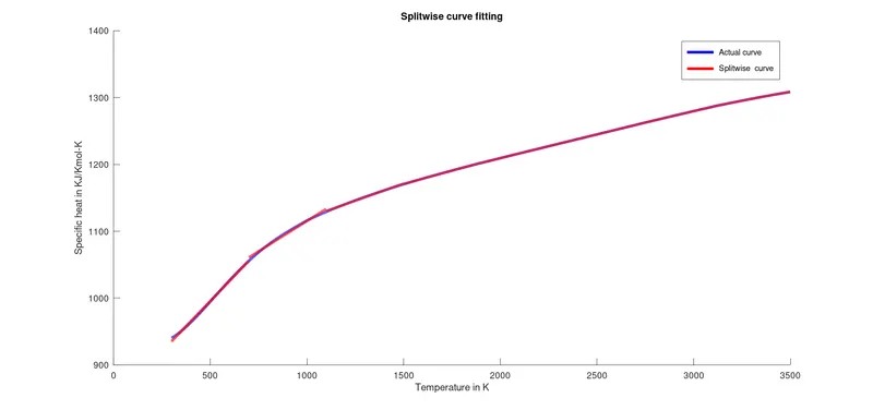
As usual, to begin our code, we need to give our input values. The input values are nothing but our gathered set of data. Herein, they are the values of specific heat against a temperature range from 300-3499 Kelvin. Therefore, as an input we need to load this data into some variable, which in our case is cp_data. Next, we have extracted the two different variables of the data set into two separate arrays (cp and temperature), for our convenience. Moving ahead, we will be making use of the polyfit function. polyfit in Matlab takes the input values of independent and dependent variables of our data along with the highest degree of the polynomial and returns the coefficients of the best fit curve. Yes, indeed it makes life that easy for us. The next function i.e polyval takes these coefficients along with the independent variables as inputs and gives our predicted values of the dependent variable (i.e the function values at various values of x). On plotting these values alongside our original dataset we can see how well our function fits the given set of data. Going ahead, we can even know the values of our curve parameters to make a conclusion about the fitness of the curve. For our problem statement, we have made use of the R-square and adjusted R-square values. Also, we have implemented the split wise method of curve fitting, wherein, we have split our data into smaller groups and then calculated the predicted values for each group. Then, on plotting these values against our original dataset we get a better fit for the same degree of polynomial as compared to the complete data treated as a whole.

The Code

%Curve fitting
close all
clear all
clc

%Load available raw data set into a variable
cp_data=load('data');

%Segregating dependent and independent variables into separate arrays
temperature=cp_data(:,1);
cp=cp_data(:,2);


% Finding coefficients corresponding to the best fit value using polyfit function
%Linear polynomial coefficients
linear_coeff = polyfit(temperature,cp,1)
%Cubic polynomial coefficients
cubic_coeff=polyfit(temperature,cp,3)

% Calculating predicted dependent variable values corresponding to coefficients obtained above using polyval
cp_predicted1= polyval(linear_coeff,temperature);
cp_predicted2= polyval(cubic_coeff,temperature);

 %Calculating goodness of fit curve parameters
 % Linear fit
for i=1:length(cp)
  x(i) = (cp_predicted1(i)-cp(i))^2;
  y(i)= (cp_predicted1(i)-mean(cp))^2;
end

%Sum of squares due to errors
SSE = sum(x);

%Sum of squares of regression
SSR = sum(y);

% R-Square
R_square = SSR/(SSR+SSE)

%Adjusted R-square
% n= number of datapoints
n=length(cp);
% k= number of independent variables
k=1;

AdjR_square = 1-(((1-R_square)*(n-1))/(n-k-1))

 if (AdjR_square>0.95)
   disp('Predicted curve is a good fit')
 else
     disp('Predicted curve is not a good fit')
 end

% Cubic fit
  for i=1:length(cp)
  x(i) = (cp_predicted2(i)-cp(i))^2;
  y(i)= (cp_predicted2(i)-mean(cp))^2;
end

%Sum of squares due to errors
SSE = sum(x);

%Sum of squares of regression
SSR = sum(y);

% R-Square
R_square = SSR/(SSR+SSE)

%Adjusted R-square
% n= number of datapoints
n=length(cp);
% k= number of independent variables
k=4;

AdjR_square = 1-(((1-R_square)*(n-1))/(n-k-1))

if (AdjR_square>0.95)
  disp('Predicted curve is a good fit')
else
  disp('Predicted curve is not a good fit')
  end
  

  %Plotting
  hold on
  plot(temperature,cp,'linewidth',3,'color','b')
hold on
title('Linear curve fitting')
plot(temperature,cp_predicted1,'linewidth',3,'color','r')
title('Cubic curve fitting')
plot(temperature,cp_predicted2,'linewidth',3,'color','g')
xlabel('Temperature in K')
ylabel('Specific heat in KJ/Kmol-K')
legend('Actual curve','Linear curve','Cubic curve')

%%
%Splitwise method (8 splits)
cp_data=load('data');
temperature=cp_data(:,1);
cp=cp_data(:,2);
% First set
temperature1= cp_data(1:400,1);
cp1 = cp_data(1:400,2);
linear_coeff1 = polyfit(temperature1,cp1,1);
cp1_predicted = polyval(linear_coeff1,temperature1);

% Second set
temperature2= cp_data(401:800,1);
cp2 = cp_data(401:800,2);
linear_coeff2 = polyfit(temperature2,cp2,1);
cp2_predicted = polyval(linear_coeff2,temperature2);

% Third set
temperature3= cp_data(801:1200,1);
cp3 = cp_data(801:1200,2);
linear_coeff3 = polyfit(temperature3,cp3,1);
cp3_predicted = polyval(linear_coeff3,temperature3);

% Fourth set
temperature4= cp_data(1201:1600,1);
cp4 = cp_data(1201:1600,2);
linear_coeff4 = polyfit(temperature4,cp4,1);
cp4_predicted = polyval(linear_coeff4,temperature4);

% Fifth set
temperature5= cp_data(1601:2000,1);
cp5 = cp_data(1601:2000,2);
linear_coeff5 = polyfit(temperature5,cp5,1);
cp5_predicted = polyval(linear_coeff5,temperature5);

% Sixth set
temperature6= cp_data(2001:2400,1);
cp6 = cp_data(2001:2400,2);
linear_coeff6 = polyfit(temperature6,cp6,1);
cp6_predicted = polyval(linear_coeff6,temperature6);

% Seventh set
temperature7= cp_data(2401:2800,1);
cp7 = cp_data(2401:2800,2);
linear_coeff7 = polyfit(temperature7,cp7,1);
cp7_predicted = polyval(linear_coeff7,temperature7);

%Eighth set
temperature8= cp_data(2801:3200,1);
cp8 = cp_data(2801:3200,2);
linear_coeff8 = polyfit(temperature8,cp8,1);
cp8_predicted = polyval(linear_coeff8,temperature8);

New_temperature = [temperature1,temperature2,temperature3,temperature4,temperature5,temperature6,temperature7,temperature8];
New_cp = [cp1_predicted,cp2_predicted,cp3_predicted,cp4_predicted,cp5_predicted,cp6_predicted,cp7_predicted,cp8_predicted];

for i=1:length(cp)
  x(i) = (New_cp(i)-cp(i))^2;
  y(i)= (New_cp(i)-mean(cp))^2;
end

%Sum of squares due to errors
SSE = sum(x);

%Sum of squares of regression
SSR = sum(y);

% R-Square
R_square = SSR/(SSR+SSE)

%Adjusted R-square
% n= number of datapoints
n=length(cp);
% k= number of independent variables
k=1;

AdjR_square = 1-(((1-R_square)*(n-1))/(n-k-1))

if (AdjR_square>0.95)
  disp('Predicted curve is a good fit')
else
  disp('Predicted curve is not a good fit')
  end

%Plotting
hold on
plot(temperature,cp,'linewidth',3,'color','b')
plot(New_temperature,New_cp,'linewidth',3,'color','r')
title('Splitwise curve fitting')
xlabel('Temperature in K')
ylabel('Specific heat in KJ/Kmol-K')
legend('Actual curve','Splitwise  curve')

Output

Linear fit

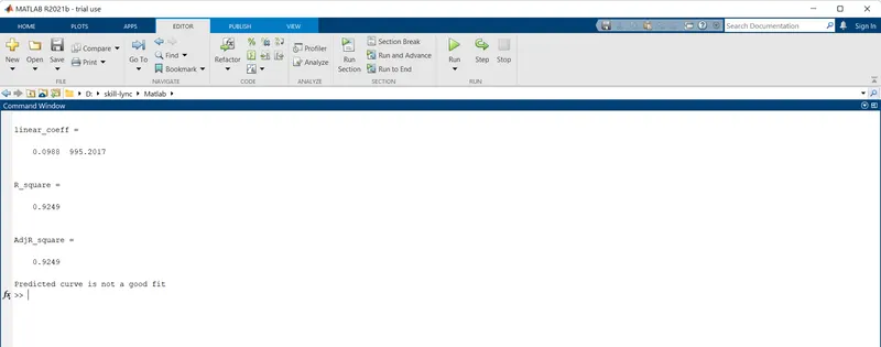
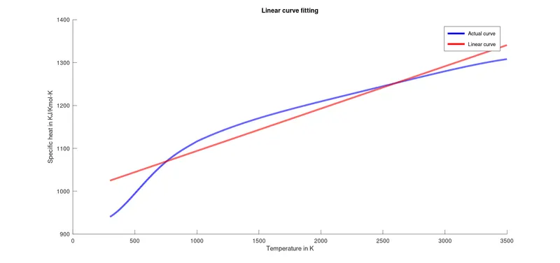
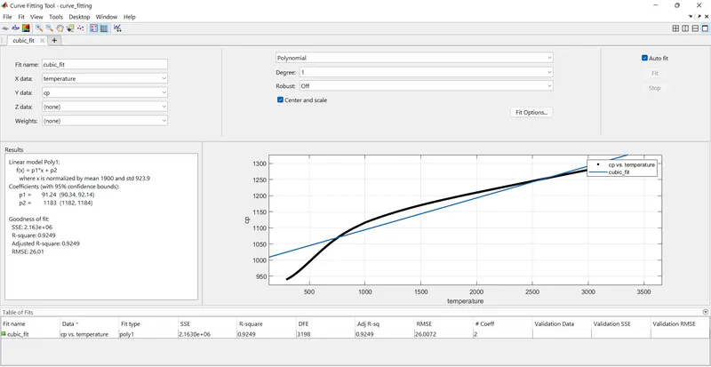
Cubic fit

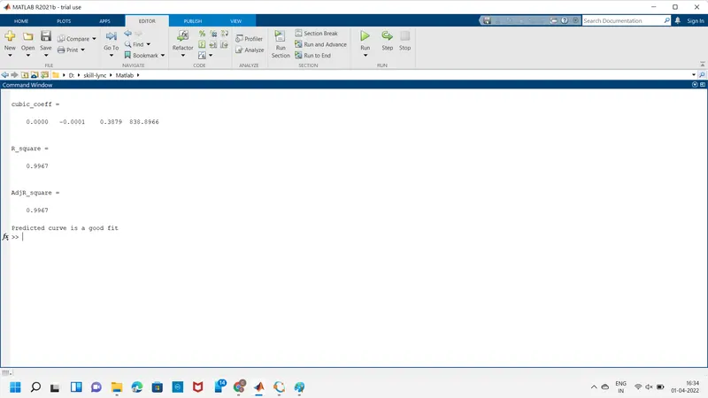
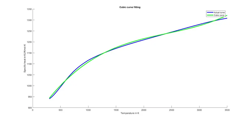
Splitwise method

References

Curve-Fitting-and-criterion-to-choose-best-fit

Evaluating-goodness-of-fit

iiserpune bhasbapat curvefitting