Challenge Week 3-Matlab code to solve ODE for simple pendulum with damping

Challenge on Second Order ODE’s

Aim: To write a program in MATLAB which solves the ODE that represents the equation of motion of a simple pendulum with damping.

The ODE for the same is given by:

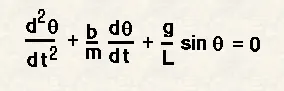
where,

g = acceleration due to gravity in m/s²,

L = length of the string of the pendulum in m,

m = mass of the object attached to the string (a ball in our case) in kg,

b=damping coefficient.

For, the case of our problem the values for the above quantities are taken to be,

g = 9.81 m/s²,

L = 1 m,

m = 1 kg,

b = 0.15.

Objectives:

1) To find solutions for the ODE for a time span of 40 sec with the initial angular displacement and angular velocity being 0 and 3 respectively.

2) To create an animation of the motion of the pendulum as a function of the ODE.

Understanding the Code:

So, we are required to write a code in MATLAB that shall give us the solution of an ODE of the above form. To do this we will make use of the ode45 command in matlab. Let's know about the function in brief, before going ahead:

Ode45 is a function in Matlab that solves ordinary or partial differential equations using a numerical method. The numerical method in question here is the 4^th order Runge-Kutta method. Runge-Kutta is a first order ODE solver for initial value problems. That is, provided an initial condition; we will be able to use the 4^th order method to solve for the solution. The ode45 function takes 3 inputs. The 3 inputs are the function to be integrated, the time span, and the initial conditions. The function could be any function while the time span would be the integration limits. This can be provided as a vector of two 2 values, the initial and the final time or with a spacing using the linspace function. The solver will choose a step size that is most suitable for the solution to obtain a result in the most optimal time possible. The initial condition would be the value of the function at time t=0 s.

The function can be provided in the form of an anonymous function,

[t,results]= ode45(@(x) x^2, tspan, y0)

Here, we don’t know the value of x and x is an input to the anonymous function that we have defined here. This is similar to defining a function that takes the input of x and gives the output of x^2. The function can also be defined as a separate function. This function must take at least two inputs, which should be t and y, apart from other arguments, where t would be the current time and y would be the value of the function at the previous time step.

Let’s consider a function ode_func; the function must be defined as,

function [output] = ode_func(t,y,args)

where args refer to any other input arguments required by the ODE.

This very function can then be called upon in the ODE as,

[t,results] = ode45(@(t,y) ode_func(t,y,args),tspan,y0)

The catch here though is that the Runge-Kutta method mentioned above is a first order solver and hence we need to provide our ODE of any order to ode45 as a set of first order ODEs.

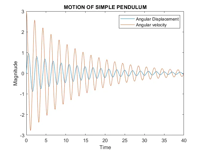
Moving on to our code syntax. Firstly, we have provided the parameter values for the various constant parameters in our ODE. In addition, we have provided the initial conditions, which is a requisite, and the time span against which we want a solution to our ODE. Then, we have defined a function ode_func which carries all the details of our ODE broken down into two first order ODE’s i.e dƟ1/dt & dƟ2/dt. Further, we implement our ode45 function as discussed above. We then plot angular displacement and angular velocity, which are the solutions of our ODE against time; with the x-axis corresponding to time values and the y-axis corresponding to the magnitudes of angular displacement and angular velocity.

For the animation part, we would require two coordinate positions each, for x and y. For the pendulum, one point is fixed and the motion of the pendulum happens about this point. Here, we have considered our origin to be this point. The other end of the pendulum has coordinates corresponding to product of sine and cosine of angular displacement values (obtained as the first column in our solution of ODE) and the length of the string, for x and y coordinates respectively. On plotting the above coordinate values for the given time span we can obtain an animation of a simple pendulum which can be stored as a movie as well.

The Code:

% Inputs

b=0.15;
m=1;
l=1;
g=9.81;
x0=0;
y0=0;

theta_0=[0;3];
t_span = linspace(0,40,500);

% Solver function
[t,results] = ode45(@(t,theta) ode_func(t,theta,b,g,l,m),t_span,theta_0);

% Plotting angular displacement and angular velocity against time 
plot(t,results(:,1))
hold on
plot(t,results(:,2))
xlabel('Time')
ylabel('Magnitude')
title('MOTION OF SIMPLE PENDULUM')
legend('Angular Displacement','Angular velocity')
hold off
results1=results(:,1);

%%
% Animating the motion of the pendulum and storing

ct=1;
for i=1:length(t_span)
    % End coordinate values
  x1=-(l*sin(results1(i)));
  y1=-(l*cos(results1(i)));
  plot([-0.5 0.5],[0 0],'linewidth',4,'Color','r')
  hold on
  plot ([x0 x1],[y0 y1],'linewidth',3,'Color','b')
  hold on
  plot(x1, y1,'-o','markersize',25,'MarkerFaceColor','g')
  axis([-1 1 -1.5 1])
  title('Animation of Simple Pendulum')
  pause(.03)
  hold off
  M(ct)=getframe(gcf);
 
  ct=ct+1;
end 

movie(M)
videofile = VideoWriter('Pendulum','Uncompressed AVI')
open(videofile)
writeVideo(videofile,M)
close(videofile)


% ode_func
function [dtheta_dt] = ode_func(t,theta,b,g,l,m)
  theta1=theta(1);
  theta2=theta(2);
  dtheta1_dt=theta2;
  dtheta2_dt=-(b/m)*theta2-(g/l)*sin(theta1);
  dtheta_dt=[dtheta1_dt;dtheta2_dt];
  end

Output:

Youtube Video Link: https://www.youtube.com/watch?v=g0U6f1Pmj4c