Project - Position control of mass spring damper system
AIM :
To design the project of position control of mass spring damper system using matlab simulink model of transfer function of a mass spring damper system and use it in the model. Add a PID controller to adjust the force on mass so that its position follows a reference signal. Using m = 3.6; %kg k = 400; %N/m c = 100; %Ns/m these values for reference.
Objective :
- Transfer function of a mass spring damper system and use it in the model. Add a PID controller to adjust the force on mass so that its position follows a reference signal. the matlab model of the pid control and transfer function pulse wavefrome generator.
- This example shows a controlled mass-spring-damper. A controller adjusts the force on the mass to have its position track a command signal. The initial velocity for the mass is 10 meters per second. The controller adjusts the force applied by the Force Source to track the step changes to the input signal.
- he mass-spring-damper model consists of discrete mass nodes distributed throughout an object and interconnected via a network of springs and dampers. This model is well-suited for modeling objects with complex material properties such as nonlinearity and viscoelasticity. Packages such as MATLAB may be used to run simulations of such models. As well as engineering simulation, these systems have applications in computer graphics and computer animation.
- The spring-mass-damper system consists of a mass with weight (m), a spring with stiffness (k), and a shock absorber with a damping coefficient of (c). This system works based on Newton’s second law, which states that Force is equal to the rate of change of momentum. For a constant mass, force equals mass times acceleration.
- Deriving the Mass Spring Damper System based on Newton’s second law F = m*a
where
F = Resultant of all the forces
m = Mass
a = Acceleration
PID controller
- A PID controller is an instrument used in industrial control applications to regulate temperature, flow, pressure, speed and other process variables. PID (proportional integral derivative) controllers use a control loop feedback mechanism to control process variables and are the most accurate and stable controller.
- A proportional–integral–derivative controller (PID controller or three-term controller) is a control loop mechanism employing feedback that is widely used in industrial control systems and a variety of other applications requiring continuously modulated control.
- PID control is a well-established way of driving a system towards a target position or level. It's a practically ubiquitous as a means of controlling temperature and finds application in myriad chemical and scientific processes as well as automation. PID control uses closed-loop control feedback to keep the actual output from a process as close to the target or setpoint output as possible.
- A digital PID controller reads the sensor signal, normally from a thermocouple or RTD and connects the measurement to engineering units, such as degree Fahrenheit or Celsius, that are then displayed in a digital format.
- We will now look at the effects of varying the Proportional component of the controller’s output, and of introducing Integral (I) and Derivative (V) terms.
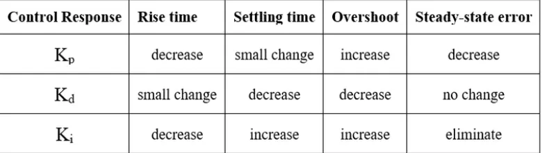
- If we have just a Proportional (P) controller, we can start by setting the Kp gain to a modest value, such as 10 (K is dimensionless). After applying the step input, the output will be stable, but will approach the desired value slowly. If Kp is increased to, say, 100, both the steady state error and the rise time will be reduced – so far, so good. However, if we increase Kp to 200, although the rise time and steady state error are further reduced, overshoot starts to appear.
- From here on, further increasing Kp merely increases overshoot, with no further reductions in rise time or steady state error. And overshoot may eventually become underdamped oscillation, meaning that the system will be unstable.
- The industry’s solution to this has been to add Integral (I) and Derivative (V) components to the controller’s Proportional (P) output, to build a PID controller.
PID controller in this project
- In this project, PID controller has been designed by using Simulink in order to control a mass spring damper system which can move any direction. A transfer function for dc motor was added on the diagram. Response curve of the PID controller were fixed by tuning.
- The computer interface, different control algorithms can be performed on the system easily; control parameters can be set up online, filter algorithms in various structures can be tried and the reaction of these changeable values to the system can be observed.
- The effects of controller Proportional Integral Derivative (PID) for developing.
Spring Mass Damper
- Spring-mass-damper theory applies the basic physics of F=ma to define suspension motion and response on bump impacts. Force (F) acting on the suspension is the combination of spring plus damping force. Mass (m) is the chassis or wheel weight depending on which body you want to look at. The combination of force and mass define the F=ma acceleration, which in turn defines the velocity, position and suspension response characteristics at any instant in time.
- Spring force: Spring force is defined by the spring constant (k) multiplied by the displacement (dy)
- Mass: Mass of the wheel or mass of the chassis. Spring-mass-damper theory describes motion of either body
- Damping: The shock absorber damping coefficient defined as damping force divided by shaft velocity. Damping linearly increases with shaft velocity
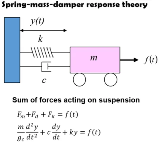
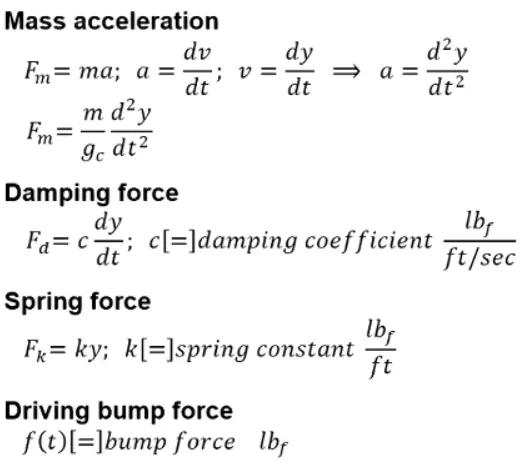
Spring-mass-damper theory applies the basic physics of F=ma to describe suspension motion
- The three forces of spring, mass and damping completely describe suspension motion. Springs make the suspension bounce up and down. Damping stops the bouncing motion. There are no other forces acting on the suspension. In that sense the spring-mass-damper system equation provides an exact description of suspension motion.
- Combining the above terms describing the forces acting on the suspension gives a single equation describing the F=ma suspension motion. The f(t) term is an arbitrary external force that kicks the suspension into motion, like hitting a bump.
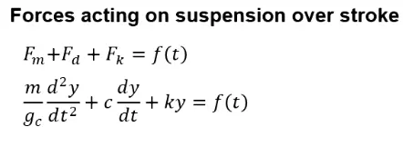
Suspension response
- The above equation can be solved analytically to obtain an exact mathematical equation describing the suspension position y(t) at any instant in time. The y(t) solution for an under damped suspension (zeta <1) is shown below.
- The suspension velocity continuously changes through the stroke, which changes the damping force. The spring force also changes with stroke position. Multiple simultaneously changing forces makes it hard to guess the suspension motion.
- Spring-mass-damper theory simplifies that complex problem identifying there are only two parameters that control suspension motion:
- tau defines the suspension oscillation frequency and the time required for the suspension to return to race sag.
- zeta describes how quickly oscillations damp.
- The suspension motion equation describes the time required for the suspension to complete one oscillation cycle, which defines the suspension damped natural resonance frequency.
TRANSFER FUNCTION :
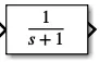
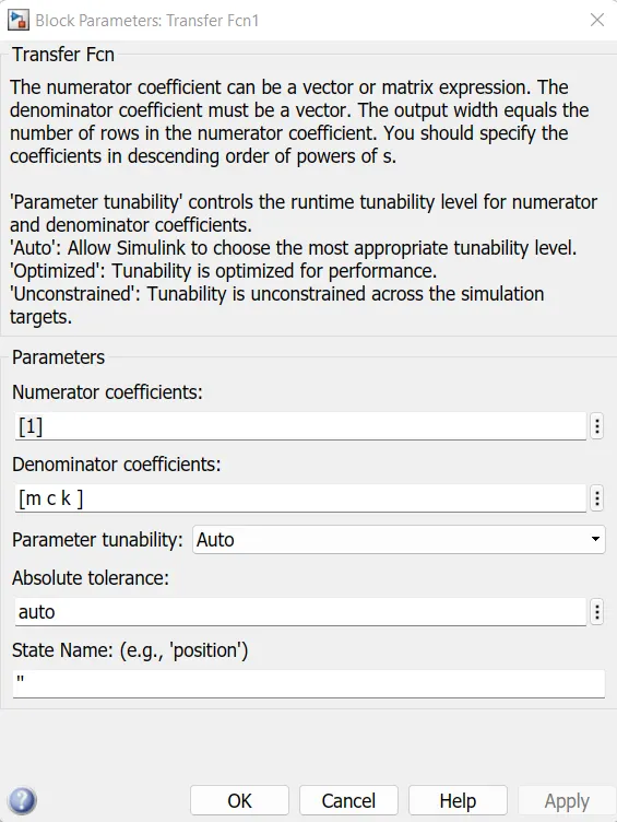
- The numerator coefficient can be a vector or matrix expression. The denominator coefficient must be a vector. The output width equals the number of rows in the numerator coefficient. You should specify the coefficients in descending order of powers of s.
- 'Parameter tunability' controls the runtime tunability level for numerator and denominator coefficients. 'Auto': Allow Simulink to choose the most appropriate tunability level. 'Optimized': Tunability is optimized for performance. 'Unconstrained': Tunability is unconstrained across the simulation targets.
- Simulink model
Transfer function of a mass spring damper system using PID controller.
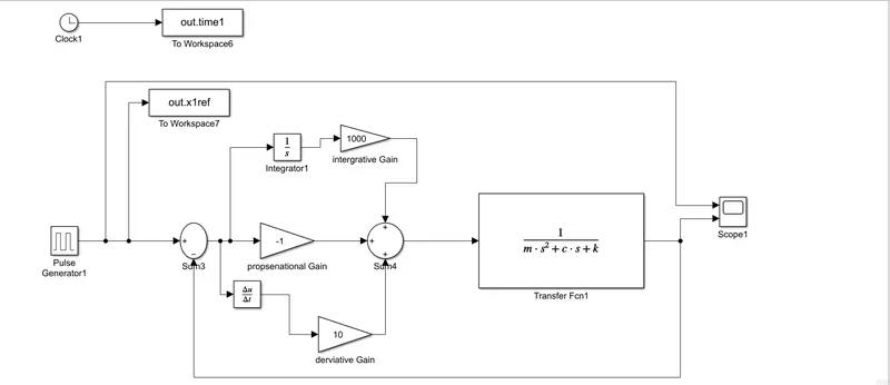
Blocks used in simulink model
- Pulse genereator :
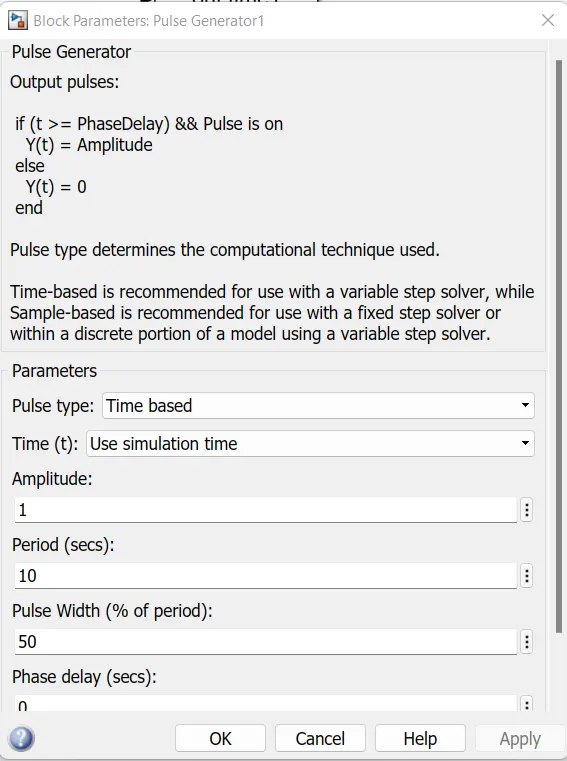
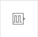 The Pulse Generator block generates square wave pulses at regular intervals. The block waveform parameters, Amplitude, Pulse Width, Period, and Phase delay, determine the shape of the output waveform. The following diagram shows how each parameter affects the waveform. The Pulse Generator block can emit scalar, vector, or matrix signals of any real data type. To emit a scalar signal, use scalars to specify the waveform parameters. To emit a vector or matrix signal, use vectors or matrices, respectively, to specify the waveform parameters. Each element of the waveform parameters affects the corresponding element of the output signal. For example, the first element of a vector amplitude parameter determines the amplitude of the first element of a vector output pulse. All the waveform parameters must have the same dimensions after scalar expansion. The data type of the output is the same as the data type of the Amplitude parameter.
 - Sum :
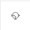 The Sum block performs addition or subtraction on its inputs. The Add, Subtract, Sum of Elements, and Sum blocks are identical blocks. This block can add or subtract scalar, vector, or matrix inputs. It can also collapse the elements of a signal and perform a summation.
You specify the operations of the block with the List of signs parameter with plus (
+), minus (-), and spacer (|).-
The number of
+and-characters equals the number of inputs. For example,+-+requires three inputs. The block subtracts the second (middle) input from the first (top) input, and then adds the third (bottom) input. -
A spacer character creates extra space between ports on the block icon.
-
If performing only addition, you can use a numerical value equal to the number of inputs.
-
If only there is only one input port, a single
+or-adds or subtracts the elements over all dimensions or in the specified dimension.
The Sum block first converts the input data type to its accumulator data type, then performs the specified operations. The block converts the result to its output data type using the specified rounding and overflow modes.
-
- Workspace :
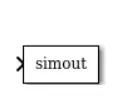 The To Workspace block writes input signal data to a workspace. During simulation, the block writes data to an internal buffer. When you pause the simulation or the simulation completes, that data is written to the workspace. Data is not available until the simulation pauses or stops.
The To Workspace block typically writes data to the MATLAB® base workspace. For a
simcommand in a MATLAB function, the To Workspace block sends data to the workspace of the calling function, not to the MATLAB base workspace. To send the logged data to the base workspace, use anassignincommand in the function. - Derivative :
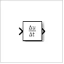 The Derivative block approximates the derivative of the input signal u with respect to the simulation time t. You obtain the approximation. The Derivative block output might be sensitive to the dynamics of the entire model. The accuracy of the output signal depends on the size of the time steps taken in the simulation. Smaller steps allow for a smoother and more accurate output curve from this block. However, unlike with blocks that have continuous states, the solver does not take smaller steps when the input to this block changes rapidly. Depending on the dynamics of the driving signal and model, the output signal of this block might contain unexpected fluctuations. These fluctuations are primarily due to the driving signal output and solver step size.
5. Gain :
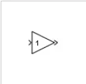 The Gain block multiplies the input by a constant value (gain). The input and the gain can each be a scalar, vector, or matrix.
You specify the value of gain in the Gain parameter. The Multiplication parameter lets you specify element-wise or matrix multiplication. For matrix multiplication, this parameter also lets you indicate the order of the multiplicands.
Gain is converted from doubles to the data type specified in the block mask offline using round-to-nearest and saturation. The input and gain are then multiplied, and the result is converted to the output data type using the specified rounding and overflow modes.
6.Transfer function:
7.Scope:
 The Time Scope is optimized for discrete time processing. The Scope is optimized for general time-domain simulation. For a side-by-side comparison.
Oscilloscope features:
-
Triggers — Set triggers to sync repeating signals and pause the display when events occur.
-
Cursor Measurements — Measure signal values using vertical and horizontal cursors.
-
Signal Statistics — Display the maximum, minimum, peak-to-peak difference, mean, median, and RMS values of a selected signal.
-
Peak Finder — Find maxima, showing the x-axis values at which they occur.
-
Bilevel Measurements — Measure transitions, overshoots, undershoots, and cycles.
You must have a Simscape™ or DSP System Toolbox license to use the Peak Finder, Bilevel Measurements, and Signal Statistics.
Scope display features:
-
Simulation control — Debug models from a Scope window using Run, Step Forward, and Step Backward toolbar buttons.
-
Multiple signals — Plot multiple signals on the same y-axis (display) using multiple input ports.
-
Multiple y-axes (displays) — Display multiple y-axes. All the y-axes have a common time range on the x-axis.
-
Modify parameters — Modify scope parameter values before and during a simulation.
-
Axis autoscaling — Autoscale axes during or at the end of a simulation. Margins are drawn at the top and bottom of the axes.
-
Display data after simulation — Scope data is saved during a simulation. If a scope is closed at the start of a simulation, when you open the scope after a simulation, the scope displays simulation results for attached input signals.
8.Integrator :
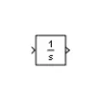
The Integrator block outputs the value of the integral of its input signal with respect to time.
Simulink® treats the Integrator block as a dynamic system with one state. The block dynamics are given by:
{˙x(t)=u(t)
x(t0) =x0
y(t) = x(t)
where:
-
u is the block input.
-
y is the block output.
-
x is the block state.
-
x0 is the initial condition of x.
While these equations define an exact relationship in continuous time, Simulink uses numerical approximation methods to evaluate them with finite precision. Simulink can use several different numerical integration methods to compute the output of the block, each with advantages in particular applications. Use the Solver pane of the Configuration Parameters dialog box (see Solver Pane) to select the technique best suited to your application.
The selected solver computes the output of the Integrator block at the current time step, using the current input value and the value of the state at the previous time step. To support this computational model, the Integrator block saves its output at the current time step for use by the solver to compute its output at the next time step. The block also provides the solver with an initial condition for use in computing the block's initial state at the beginning of a simulation. The default value of the initial condition is 0. Use the block parameter dialog box to specify another value for the initial condition or create an initial value input port on the block.
9.Clock

The Clock block outputs the current simulation time at each simulation step. This block is useful for other blocks that need the simulation time.
When you need the current time within a discrete system, use the Digital Clock block.
Explanation for simulink model
- In Gain Block Model, we used a step function. This block is connected with three different individual blocks represented as Kp, Ki & Kd.
- Here kp,kd and ki are the feedback control gains.
- As these values are already given to us, so we connected them to a sum block. Here Ki is Integrated before connecting to a Sum block whereas Kd, goes on further to perform its integrator using a filter coefficient to get the accurate variables at the end.Finally, these three individual blocks are connected to a sum block which further passes the signal to a Transfer Function and we get the desired result.
- Finally, these three individual blocks are connected to a sum block which further passes the signal to a Transfer Function and we get the desired result.
- Here we used ki gain as 1000 randomly so as to plot graph smoothly for smooth operation of dc motor.
- We used here pulse generator.
- We have connected two different models connected together i.e PID controller model and transfer function block model.
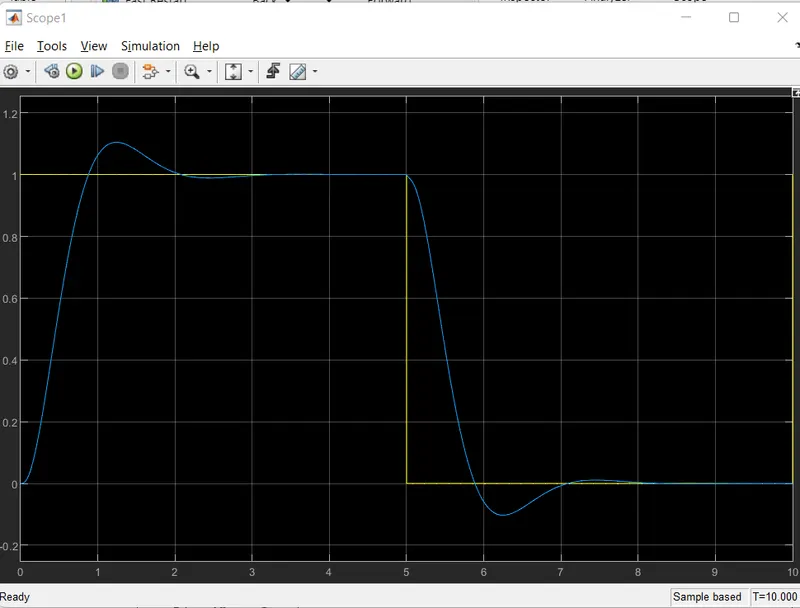
- At stop time 10secs we run the model to see observations of plot for checking settling time, overshoot, and steady-state error are met. And varied values of kp,ki,kd so as to get desired output as per reference.
Input parameters for pulse generator .
Input parameters for Transfer function.
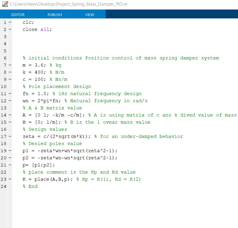
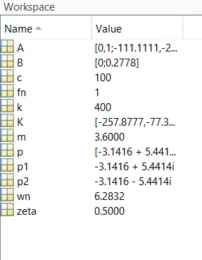
Script file:
clc;
close all;
% initial conditions Position control of mass spring damper system
m = 3.6; % kg
k = 400; % N/m
c = 100; % Ns/m
% Pole placement design
fn = 1.0; % 1Hz natural frequency design
wn = 2*pi*fn; % Natural frequency in rad/s
% A & B matrix value
A = [0 1; -k/m -c/m]; % A is using matrix of c ans k dived value of mass
B = [0; 1/m]; % B is the 1 ovear mass value
% Design values
zeta = c/(2*sqrt(m*k)); % for an under-damped behavior
% Desied poles value
p1 = -zeta*wn+wn*sqrt(zeta^2-1);
p2 = -zeta*wn-wn*sqrt(zeta^2-1);
p= [p1;p2];
% place comment is the Kp and Kd value
K = place(A,B,p); % Kp = K(1), Kd = K(2)
% End
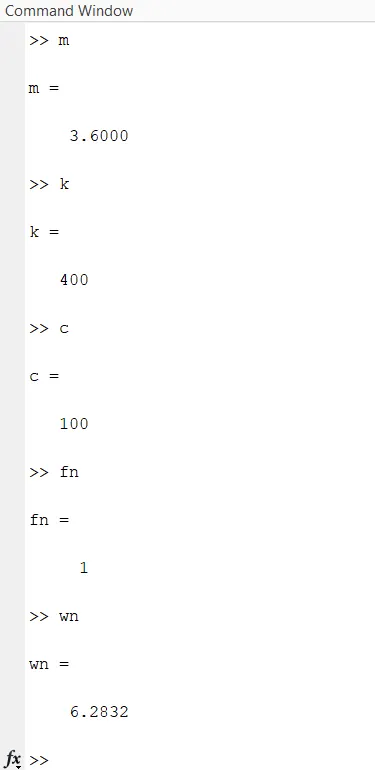
Command Window :
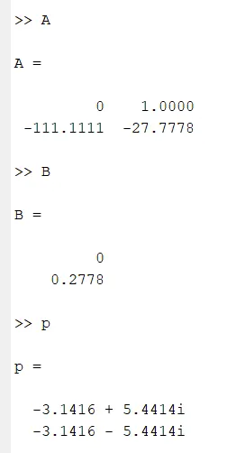
Workspace:
Matlab Simulink Model Of Position control of mass spring damper system :
- The numerator coefficient can be a vector or matrix expression. The denominator coefficient must be a vector. The output width equals the number of rows in the numerator coefficient. You should specify the coefficients in descending order of powers of s.
- 'Parameter tunability' controls the runtime tunability level for numerator and denominator coefficients. 'Auto': Allow Simulink to choose the most appropriate tunability level. 'Optimized': Tunability is optimized for performance. 'Unconstrained':Tunability is unconstrained across the simulation targets.
Result :
We have changed values of Integrative gain to 1000, Derivative gain to 10 and propsenational gain to -1.So as to reduce the spikes and generate output rectangular specified, And follow reference signal.
Wave is overshooting at nearer to 1 on x axis and undershooting at point 6.
Conclusion
To obtain the transfer function of a mass spring damper system and used it in the model.We have PID controller for using it along with the transfer function to adjust the force on mass so that its position follows a reference signal.And used different values of kp,kd,ki so as to generete the pulse as per reference wave.We have varied different values of kp,ki,kd so as to obtain desired outpt.