Project - Position control of mass spring damper system

Question:-

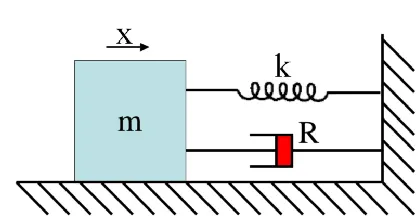
Obtain the transfer function of a mass spring damper system and use it in the model. Add a PID controller to adjust the force on mass so that its position follows a reference signal.

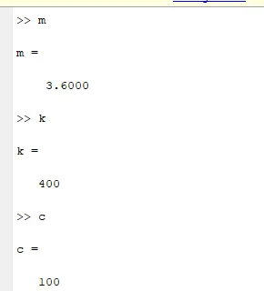
Take m = 3.6; %kg k = 400; %N/m c = 100; %Ns/m

The reference signal is shown in the following figure

Aim of the Project

Designing a position control system for a mass-spring-damper system involves several steps, including creating a Simulink model, incorporating the transfer function of the system, and adding a PID controller.

Objective:-

Create a Simulink model incorporating the transfer function of a mass-spring-damper system. Introduce a PID controller to regulate the force on the mass, aligning its position with a reference signal. The MATLAB model includes both the PID controller and the transfer function pulse waveform generator. In this demonstration, a controlled mass-spring-damper system is featured, where the controller dynamically adjusts the force on the mass to ensure its position closely follows a given command signal. The system begins with an initial velocity of 10 meters per second, and the controller adapts the applied force to track any step changes in the input signal. For the PID controller implementation:

• The Simulink environment is utilized to design and fine-tune the PID controller.
• A transfer function representing a DC motor is integrated into the model.
• The response curve of the PID controller is meticulously adjusted through tuning.

This project showcases the effectiveness of a PID controller in governing a mass-spring-damper system with multidirectional movement. The transfer function for a DC motor enriches the system's dynamics, and by tuning the PID controller, the response is optimized. The Simulink interface facilitates easy experimentation with various control algorithms, allowing online parameter setup and observing system reactions to dynamic changes. The project emphasizes the influential role of the Proportional-Integral-Derivative (PID) controller in system development.

Below is a step-by-step guide:

Step 1: Create a Simulink Model

1. Open MATLAB and Simulink.
2. Create a new Simulink model: `File > New > Simulink Model`.

Step 2: Define the Mass-Spring-Damper Transfer Function

1. Add the Mass-Spring-Damper Transfer Function Block:
2. From the Simulink Library Browser, go to `Simulink > Continuous`.
3. Drag the Transfer Function block into your model.
4. Set the Transfer Function Parameters:
5. Double-click on the Transfer Function block.
6. Set the transfer function parameters based on your mass-spring-damper system.

Step 3: Add PID Controller

1. Add a PID Controller:
2. From the Simulink Library Browser, go to `Simulink > Discrete`.
3. Drag the PID Controller block into your model.
4. Connect the Blocks:
5. Connect the output of the Transfer Function block to the input of the PID Controller.
6. Connect the output of the PID Controller to the input of the Transfer Function block.
7. Double-click on the PID Controller block to set its parameters:
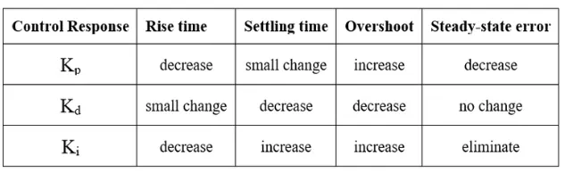
8. Adjust Proportional (P), Integral (I), and Derivative (D) gains based on your system requirements.
9. You may need to tune these parameters to achieve the desired response.

Step 4: Add Reference Signal and Scope

1. Add a Step block from the `Simulink > Sources` library to generate a reference signal.
2. Connect the Step block to the input of the system.
3. Add a Scope block from the `Simulink > Sinks` library to visualize the system's response.

Step 5: Configure Simulation Parameters

1. Configure Simulation Parameters:
2. Go to `Simulation > Model Configuration Parameters`.
3. Set the simulation time, solver type, and other parameters.

Step 6: Run the Simulation

1. Simulate by clicking the "Run" button in the Simulink toolbar.

Step 7: Analyze and Tune

1. Analyze the system's response to the Scope.
2. If necessary, adjust PID controller gains and other parameters to achieve the desired performance.

Step 8: Save and Document

1. Save your Simulink model and document the parameters and design choices.

redo iterate and refine your design based on the system's response and performance requirements. Additionally, MATLAB and Simulink provide tools for system analysis and tuning, such as the Control System Toolbox. This guide provides a basic outline, and the specific details will depend on the characteristics of your mass-spring-damper system and the desired control performance.

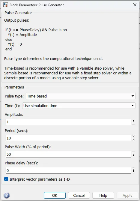
Pulse Generator:-

to generate the necessary signal we will be using a pulse generator block. so the following changes are required for the desired signal as an input

keep the amplitude to 1 change the period to 10 seconds change the pulse width to 50% we do need to change the delay

Transfer Function:-

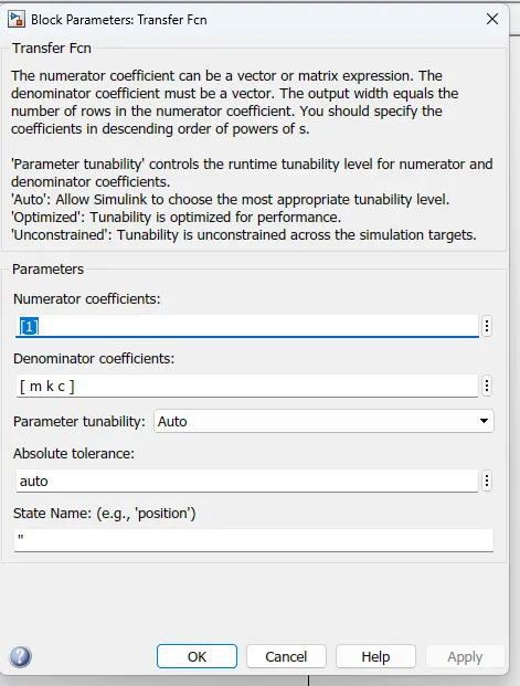
The numerator coefficient is flexible, allowing for a vector or matrix expression, while the denominator coefficient must be a vector. The number of rows in the numerator coefficient determines the output width. It is essential to specify the coefficients in descending order of powers of s.

The 'Parameter tunability' option manages the runtime tunability level for numerator and denominator coefficients. 'Auto' enables Simulink to autonomously determine the most suitable tunability level. 'Optimized' ensures tunability is optimized for performance, and 'Unconstrained' provides unconstrained tunability across simulation targets.

change the numerator to 1 keeping in a square bracket the denominator represents the KP KI And Kd so change them into mass spring and damper. those values are being defined in the script

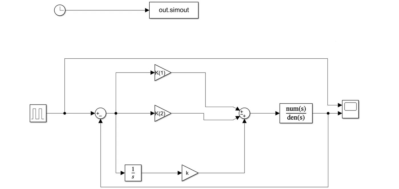
Circuit diagram:-

below is the diagram

To design a closed loop control scheme for a DC motor the following changes need to be done in the model in the previously created model. Speed is the controllable parameter, so we will set the reference speed in the step block as 10,20, 40 whichever you want. Subtract the actual speed from the reference speed to generate the error signal e(t) Add Kp as K(1) and Kd as K(2) parameter determined from the place command (K=place(A, B, P)). (use gain block to mention values of Kp, Kd, and Ki) The feedback for Kd is provided from the output current of the plant/model (figure 1). OR we can take feedback (error speed signal as input to Kd shown by figure 2) Add Ki manually with gain and integrator block tune different values of Ki and check the impact of it on results. 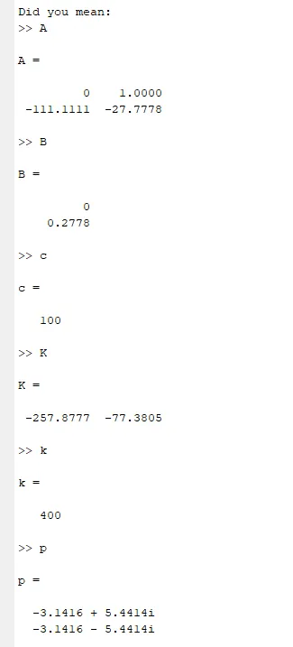To check the location of poles on the s-plane from MATLAB the following command (‘pump’-pole zero placement or mapping) can be used in continuation to the above script. You can see two crosses in red indicate complex poles lying on the left hand of the plane which indicates it is a stable system.

the script is as

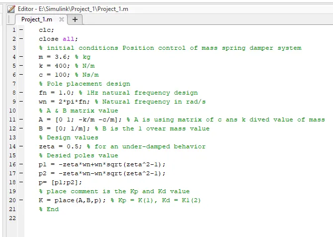CLC; close all; % initial conditions Position control of mass spring damper system m = 3.6; % kg k = 400; % N/m c = 100; % Ns/m % Pole placement design fn = 1.0; % 1Hz natural frequency design wn = 2*pi*fn; % Natural frequency in rad/s % A & B matrix value A = [0 1; -k/m -c/m]; % A is using a matrix of c ans k dived value of mass B = [0; 1/m]; % B is the 1 over mass value % Design values zeta = 0.5; % for an under-damped behavior % Desied poles value p1 = -zeta*wn+wn*sqrt(zeta^2-1); p2 = -zeta*wn-wn*sqrt(zeta^2-1); p= [p1;p2]; % place comment is the Kp and Kd value K = place(A,B,p); % Kp = K(1), Kd = K1(2) % End

Observaion:-

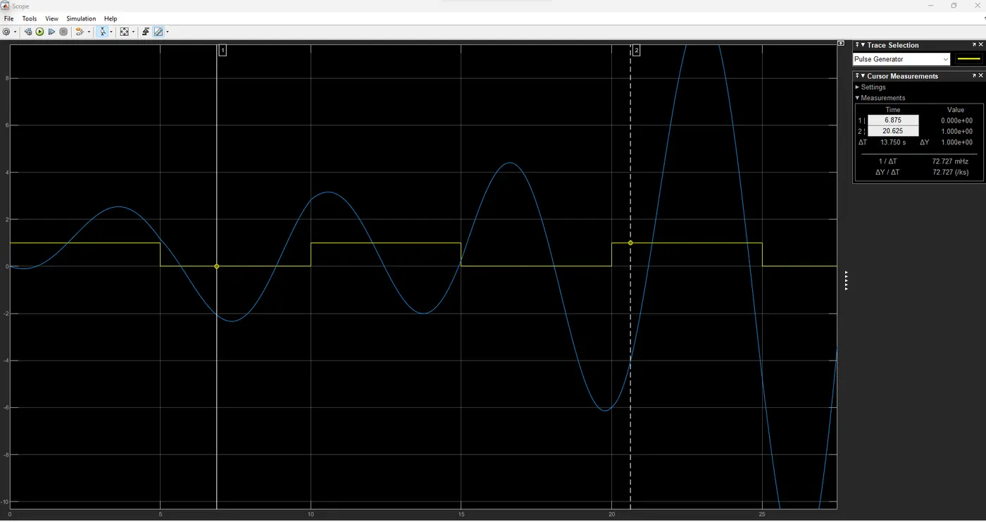
Conclusion:-

To finalize the Position Control project for a mass-spring-damper system, incorporate the transfer function of the system into the model. Integrate a PID controller to dynamically adjust the force acting on the mass, ensuring its position accurately tracks a reference signal. Implement these components using MATLAB and Simulink, and visualize the system's response through a waveform plot.