Project - Position control of mass spring damper system
AIM
Obtain the transfer function of a mass spring damper system and use it in the model. Add a PID controller to adjust the force on mass so that its position follows a reference signal.
Take m = 3.6; %kg k = 400; %N/m c = 100; %Ns/m
The reference signal is shown in the following figure.
OBJECTIVE
Given data;
Take m = 3.6; %kg k = 400; %N/m c = 100; %Ns/m
solution;
Transfer function of a mass spring damper system and use it in the model. Add a PID controller to adjust the force on mass so that its position follows a reference signal. the matlab model of the pid control and transfer function pulse wavefrome generator.
This example shows a controlled mass-spring-damper. A controller adjusts the force on the mass to have its position track a command signal. The initial velocity for the mass is 10 meters per second. The controller adjusts the force applied by the Force Source to track the step changes to the input signal.
PID controller;
PID control stands for proportional–integral–derivative control. PID control is a feedback mechanism used in a control system. This type of control is also termed as three-term control, and is implemented by a PID Controller. By calculating and controlling three parameters – the proportional, integral and derivative of how much a process variable deviates from the desired set point value – we can achieve different control actions for specific work.
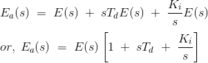
PID controllers are considered to be the best controller in the control system family. Nicholas Minorsky published the theoretical analysis paper on PID controller. For PID control the actuating signal consists of proportional error signal added with derivative and integral of the error signal. Therefore, the actuating signal for PID control is:

The Laplace transform of the actuating signal incorporating PID control is
There are some control actions which can be achieved by using any of the two parameters of the PID controller. Two parameters can work while keeping the third one to zero. So PID controller becomes sometimes PI (proportion-integral), PD (proportional-derivative) or even P or I. The derivative term D is responsible for noise measurement while the integral term is meant for reaching the targeted value of the system. In early days PID controller was used as a mechanical device. These were pneumatic controllers as they were compressed by air. Mechanical controllers include spring, lever or mass. Many complex electronic systems are provided with a PID control loop. In modern days PID controllers are used in PLC (programmable logic controllers) in the industry. The proportional, derivative and integral parameters can be expressed as – Kp, Kd and Ki. All these three parameters have an effect on the closed loop control system. It affects rise time, settling time and overshoot and also the steady state error.
| Control Response | Rise time | Settling time | Overshoot | Steady state error |
| Kp | decrease | small change | increase | decrease |
| Kd | small change | decrease | decrease | no change |
| Ki | decrease | increase | increase |
eliminate |
PID control combines the advantages of proportional, derivative and integral control actions. Let us discuss these control actions in brief.
A PID controller has some limitations also apart from being one of the best controllers in control action system. PID control is applicable to many control actions but it does not perform well in case of optimal control. Main disadvantage is the feedback path. PID is not provided with any model of the process. Other drawbacks are that PID is linear system and derivative part is noise sensitive. Small amount of noise can cause great change in the output.
The mass-spring-damper model consists of discrete mass nodes distributed throughout an object and interconnected via a network of springs and dampers. This model is well-suited for modeling objects with complex material properties such as nonlinearity and viscoelasticity. Packages such as MATLAB may be used to run simulations of such models. As well as engineering simulation, these systems have applications in computer graphics and computer animation.
The spring-mass-damper system consists of a mass with weight (m), a spring with stiffness (k), and a shock absorber with a damping coefficient of (c). This system works based on Newton’s second law, which states that Force is equal to the rate of change of momentum. For a constant mass, force equals mass times acceleration.
Deriving the Mass Spring Damper System based on Newton’s second law F = m*a
where
F = Resultant of all the forces
m = Mass
a = Acceleration
Fig1: Mass Spring Damper System in Rest
k is the spring stiffness
d is the damping coefficient
The above system is in a state of rest. Let's consider a moving Mass Spring Damper System to see forces act during motion. What are the forces acting if the system is moving?
Fig2: Mass Spring Damper System in Motion
Expression for Spring Force and Damping Force
Fs = k*x ----(1)
Fd = d*(dx/dt) ----(2)
Applying F = m*a
ΣF = m*(d^2x/dt^2) (in the positive direction)
− Fs − Fd + F = m*(d^2x/dt^2)
F = m*(d^2x/dt^2) + Fd + Fs ----(3)
Substituting eq(1) and eq(2) in eq(3)
F = m*(d^2x/dt^2) + d*(dx/dt) + k*x
The above equation is the equation of motion (EOM).
Applying Laplace Transform to the above equation
F(s) = m*(s^2*x(s)) + d*(s*x(s)) + k*x(s)
F(s) = (m*s^2 + d*s + k)*x(s)
x(s)/F(s) = 1/(m*s^2 + d*s + k)......transfer fnc
The above equation is the transfer function.
Schematic of a control system with TRAC in the adaptive outer loop
Fig (1)
Block diagram of an adaptive position control system for a spring-mass-damper system with a PI controller, full state feedback and TRAC in the adaptive outer loop
Square wave tracking of the system in Fig. 1 with the transfer functions in (15) for small (top) and large (bottom) parametric disturbances in the plant model
Model
The Simulink Model is built to obtain the transfer function of a mass spring damper system. A PID controller is also implemented into the system to adjust the force on the mass so that its position follows a reference signal.
Below are some of the block details used to create the Simulink Model,
- Pulse Generator
(Generate square wave pulses at regular intervals)
The Pulse Generator block generates square wave pulses at regular intervals. The block waveform parameters, Amplitude, Pulse Width, Period, and Phase delay, determine the shape of the output waveform. The following diagram shows how each parameter affects the waveform.
- PID Controller
(Continuous-time or discrete-time PID controller)
This block implements continuous- and discrete-time PID control algorithms and includes advanced features such as anti-windup, external reset, and signal tracking. You can tune the PID gains automatically using the 'Tune...' button (requires Simulink Control Design).
- Transfer Function
(Model linear system by transfer function)
The Transfer Fcn block models a linear system by a transfer function of the Laplace-domain variable s. The block can model single-input single-output (SISO) and single-input multiple-output (SIMO) systems.
A Pulse Generator block is used as a reference Force input signal for the system. A Transfer function block is used for the implementation of the Mass Spring Damper system. The systems-derived equation in the Laplace transform is used in the transfer function. Variables of the same are defined through a Matlab script. The output of the transfer function is the displacement of the system, which is then fed back to the PID Controller as an error signal after subtracting it from the reference signal. Using a Controller, the system throws the best tracking response.
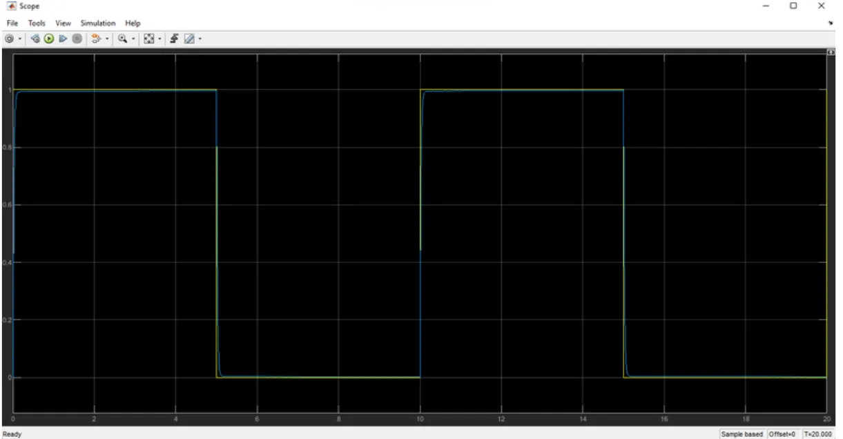
To complete the project of Position control of mass spring damper system transfer function of a mass spring damper system and use it in the model. Add a PID controller to adjust the force on mass so that its position follows a reference signal to using MATLAB and Simulink wave from plot.
SIMULINK
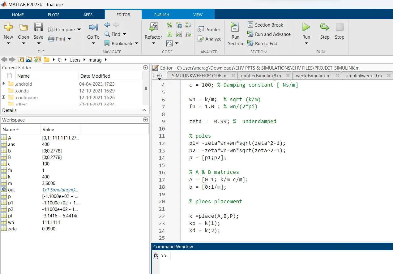
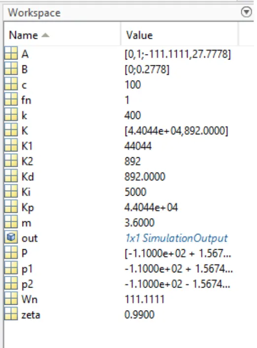
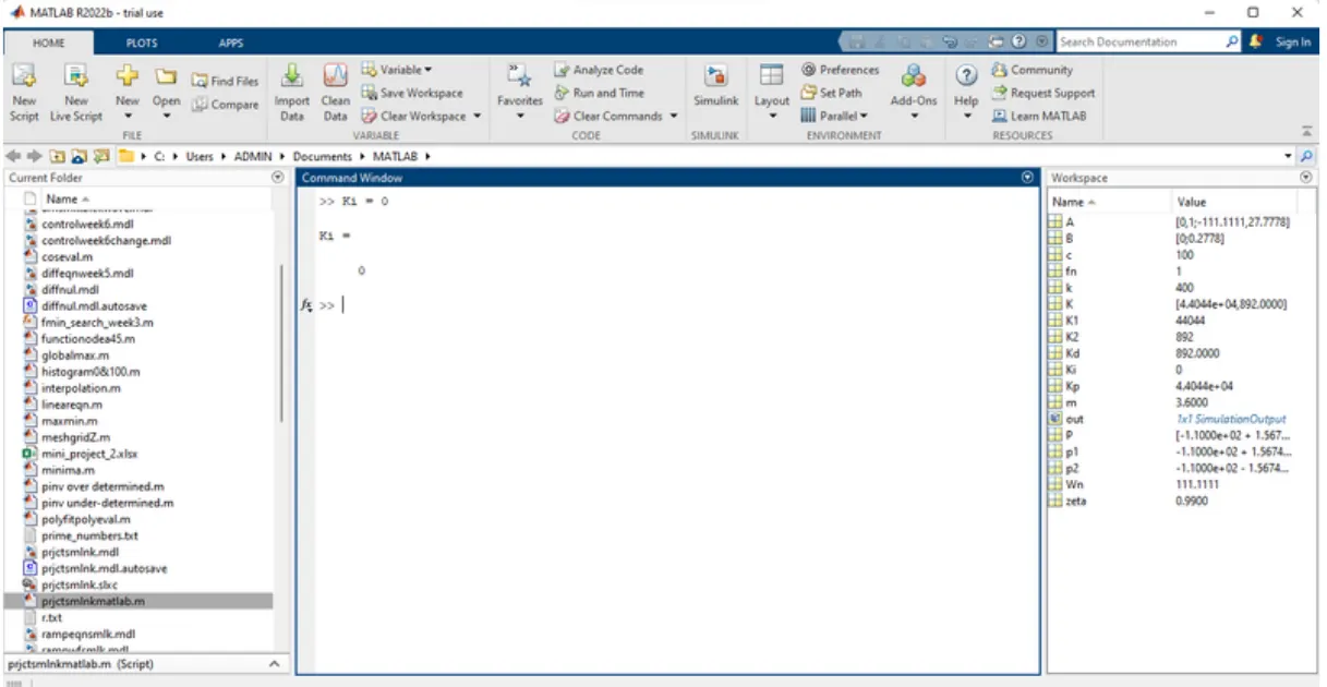
ki =0
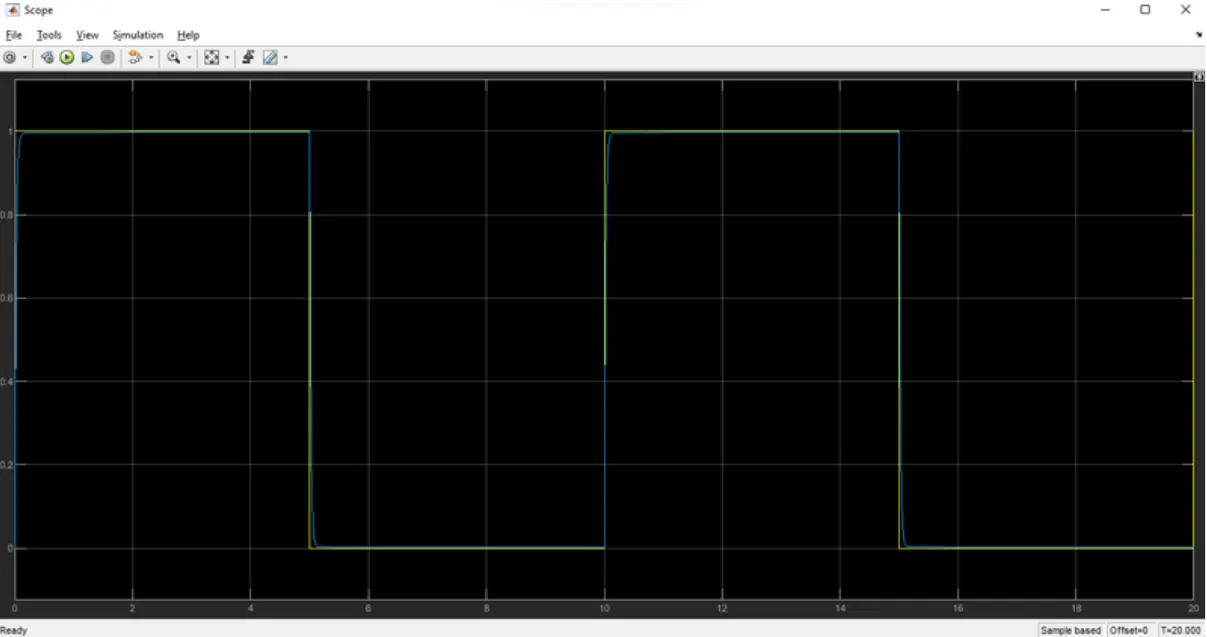
ki=5000
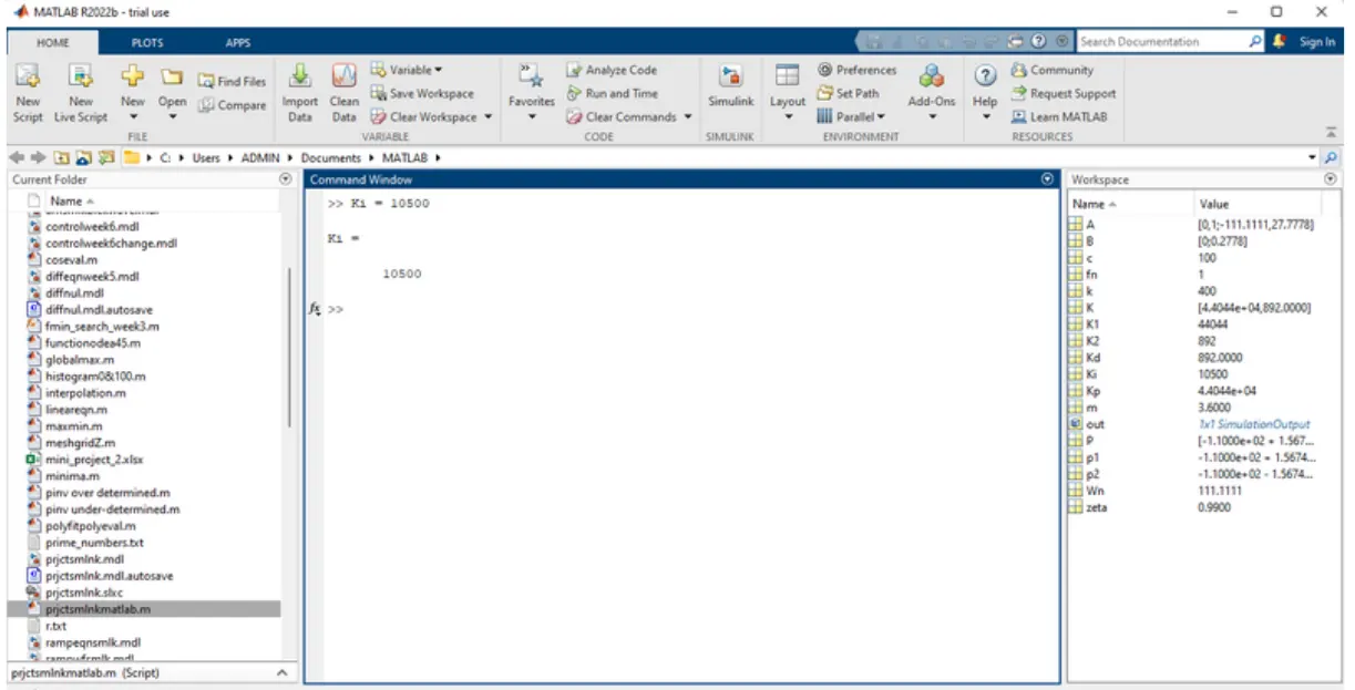
ki = 10500
CONCLUSION
To complete the project of Position control of mass spring damper system transfer function of a mass spring damper system and use it in the model. Add a PID controller to adjust the force on mass so that its position follows a reference signal to using MATLAB and Simulink wave from plot.