Project - Position control of mass spring damper system

For mass-spring system,

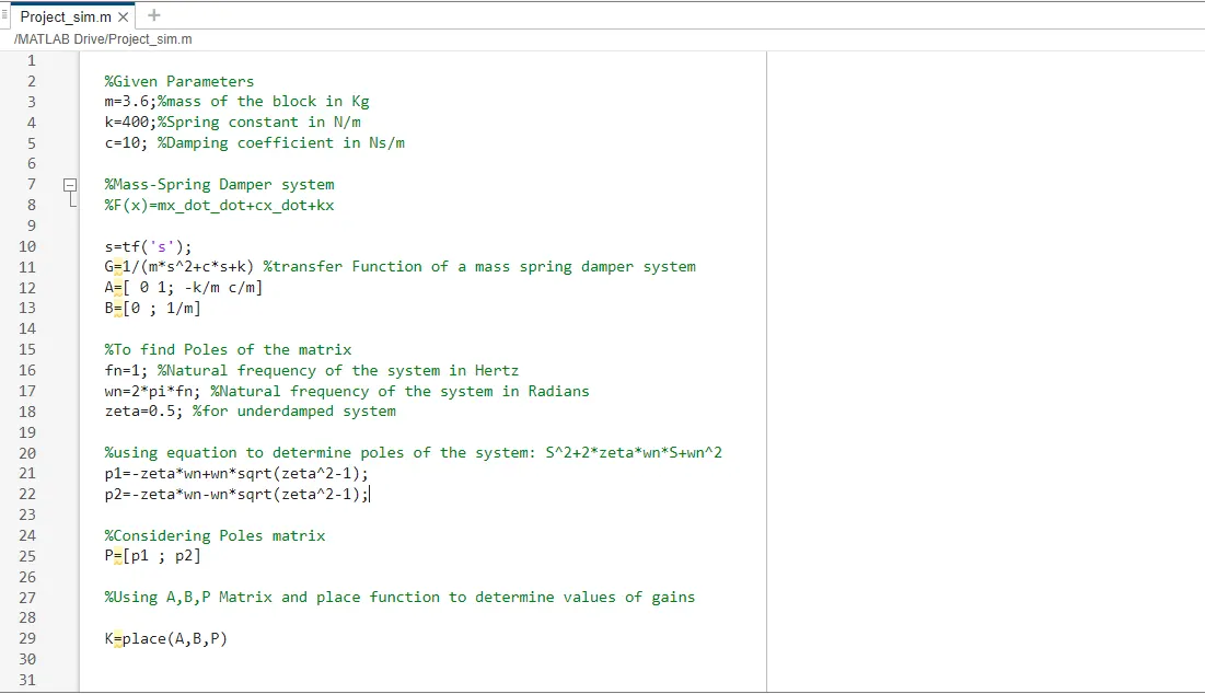
1. F(t)=m*xdot_dot + c*xdot +k*x where,

• x=displacement
• xdot=df(x)/dt,
• xdot_dot=d(xdot)/dt,
• As per the given parameters:
• m=3.6 (mass of the block in Kg)
• k=400 (spring constant of spring system in N/m)
• c=10 (damping coefficient in Ns/m)

mass-spring system in Transfer Function form:

X(s)/F(s)=1/(ms^2 +cs+k)

X(s)=[1/(ms^2 +cs+k)].F(s)

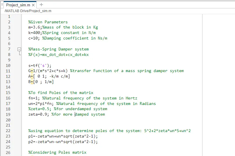
2. To find poles of the system : s^2+2*zeta*wn*s+wn^2

design parameters

• fn=1 (Natural frequency of the system in Hertz)
• Wn=2*pi*wn (Natural frequency of the system in Rad/s)
• zeta=0.5 (for underdamped system)
• p1=-zeta*wn+wn*sqrt(zeta^2-1)
• p2=-zeta*wn-wn*sqrt(zeta^2-1)

3.To find dynamics of the system using place function,

A=[ 0 1 ; -k/m c/m]

B=[ 0;1/m]

P=[p1;p2]

K=place(A,B,P)

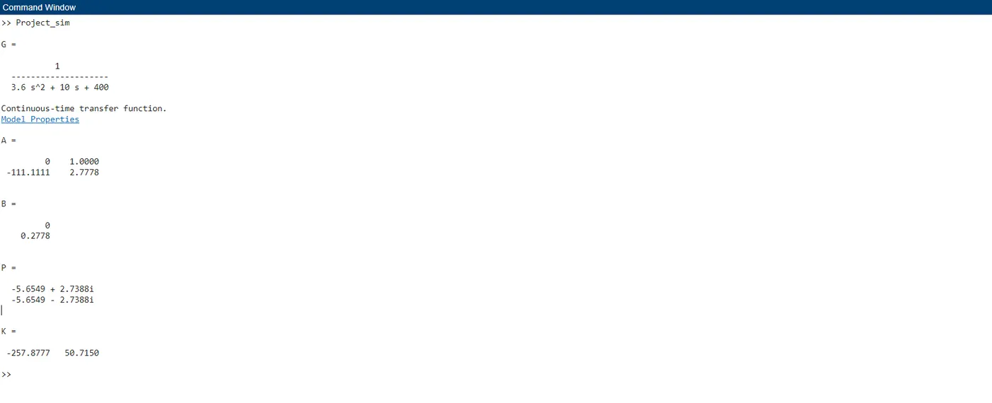
• Below is the matlab file that mentions all the parameters of the mass-spring system

 

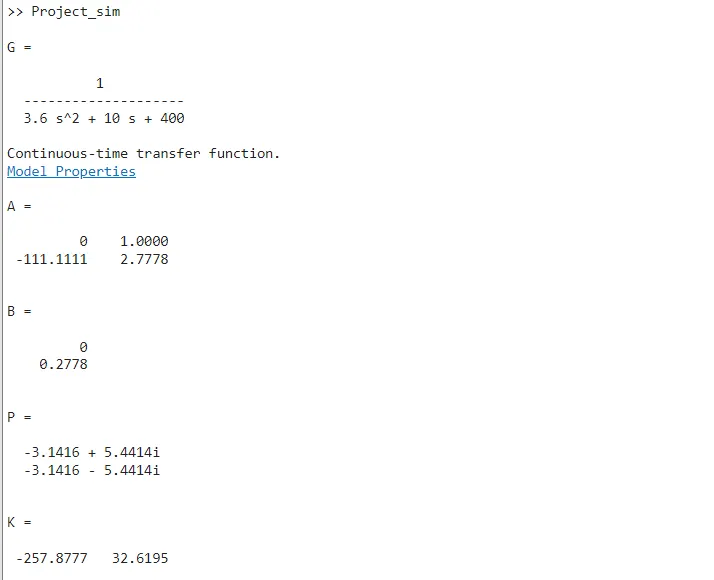
Hence, value of Kp=-257.877 & Kd=32.6195

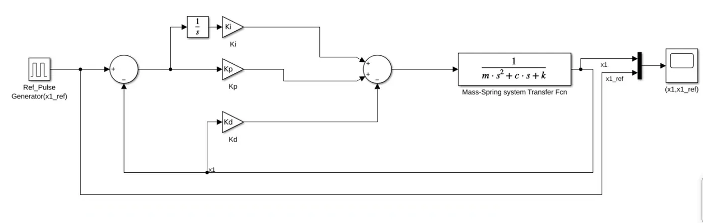
4.To Build Simulink model of mass-spring system with PID Controller

• Pulse Signal Generator : Reference signal for displacement, Magnitude=1, Pulse width=50%, Period=10secs

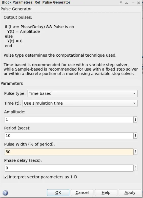
• Transfer Function Block : to represent transfer function of mass-spring system

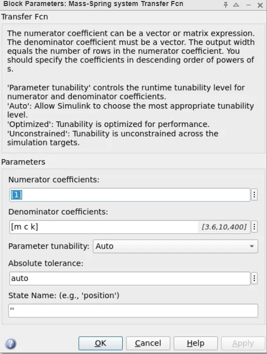
• Gain Block : For Kp,Ki,Kd gains
• Sum Block
• Scope Block : to plot xref & x signals

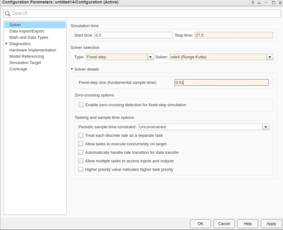
• Model Settings : Fixed Step (0.01) using Runge Kutta method(ode4) to solve the polynomial equation

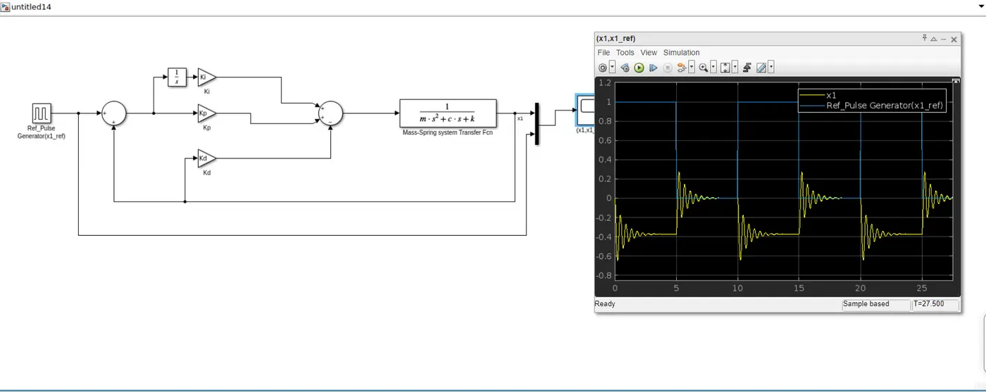
Initial Plot of x1ref & x1 with Kp=-257.877, Kd=32.6195, Ki=0;

• Observation : Response is not as per the reference pulse signal 

5.With mode damped system , zeta=0.9, and no Change in gains to observe the tracking response

• Observation : Response is not as per the reference pulse signal 

 

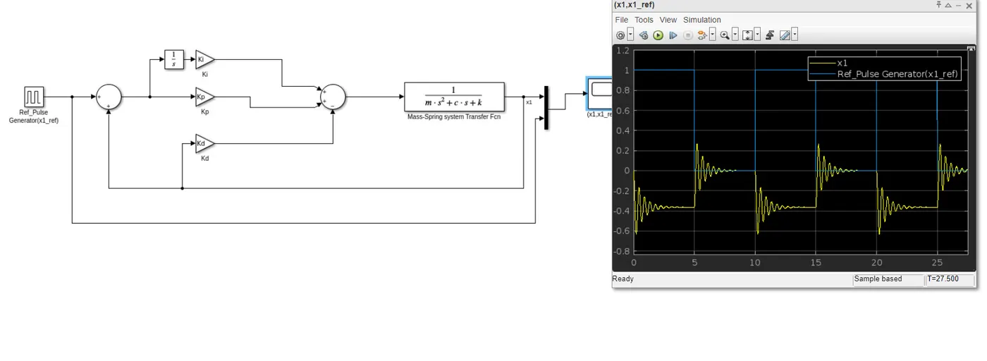
6. With Change in gains Initial Plot of x1ref & x1 with Kp=-257.877, Kd=32.6195, Ki=50,zeta=0.5;

• Observation : Response is improved than in observation 4th 

7. With Change in gains Initial Plot of x1ref & x1 with Kp=50, Kd=32.6195, Ki=100,zeta=0.5;

• Observation : Response is improved than in observation 6th 

8. With Change in gains Initial Plot of x1ref & x1 with Kp=50, Kd=32.6195, Ki=500,zeta=0.5;

• Observation : Response is improved than in observation 7th 

9. With Change in gains Initial Plot of x1ref & x1 with Kp=50, Kd=32.6195, Ki=800,zeta=0.5;

• Observation : Response is improved than in observation 8th , ess decreased, tr is improved

10. With Change in gains Initial Plot of x1ref & x1 with Kp=50, Kd=32.6195, Ki=800,zeta=0.9;

• Observation : Response is same as with zeta=0.5

11. With Change in gains Initial Plot of x1ref & x1 with Kp=50, Kd=0, Ki=800,zeta=0.9 (decrease in Kd to 0)

• Observation : in response undershoots and overshoots are observed

12. With Change in gains Initial Plot of x1ref & x1 with Kp=80, Kd=32.6195, Ki=700,zeta=0.9 

• Observation : Not much change in the response

13. With Change in gains Initial Plot of x1ref & x1 with Kp=10, Kd=32.6195, Ki=1000,zeta=0.9 

• Observation : in response undershoots and overshoots are observed

14. With Change in gains Initial Plot of x1ref & x1 with Kp=50, Kd=32.6195, Ki=800,zeta=0.9 

• Observation :response is much better

15. Final value of dynamics With Kp=50, Kd=32.6195, Ki=700,zeta=0.9

 

***Matlab files, command window and simulink model are enclosed, including plots of x1  & x1ref for different gain values