Project - Position control of mass spring damper system

Aim:

Obtain the transfer function of a mass spring damper system and use it in the model. Add a PID controller to adjust the force on mass so that its position follows a reference signal.

Take m = 3.6; %kg k = 400; %N/m c = 100; %Ns/m

Objective:

The transfer function of a mass spring damper system and its use in the model. Add a PID controller to adjust the force on mass so that its position follows a reference signal. the Matlab model of the PID control and transfer function pulse waveform generator.

This example shows a controlled mass spring damper. A controller adjusts the force on the mass to have its position track a command signal. The controller adjusts the force applied by the Force Source to track the step changes to the input signal.

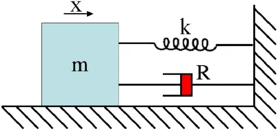
In this project, the PID controller has been designed by using Simulink in order to control a mass spring damper system that can move in any direction. A transfer function for the DC motor was added to the diagram. The response curve of the PID controller was fixed by tuning. In the computer interface, different control algorithms can be performed on the system easily; control parameters can be set up online, filter algorithms in various structures can be tried and the reaction of these changeable values to the system can be observed.

Spring mass damper system:

The mass-spring-damper model consists of discrete mass nodes distributed throughout an object and interconnected via a network of springs and dampers. This model is well-suited for modeling objects with complex material properties such as nonlinearity and viscoelasticity. Packages such as MATLAB may be used to run simulations of such models. As well as engineering simulation, these systems have applications in computer graphics and computer animation.

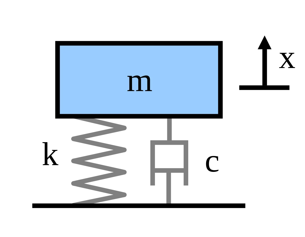
To analyze the mass-spring-damper system it is a prerequisite to understanding how to model the equations of each component with the knowledge of Newton’s 2^nd law of motion. Which are represented below.

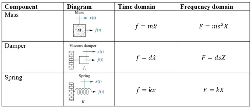
With the following points of consideration, the modeling is done.

• Point masses are present only
• is the resultant of all forces
• is absolute acceleration
• Linear force in direction is acting.

The following free body diagram (FBD) in a positive deflected state is presented.

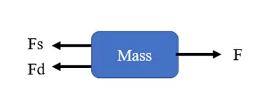
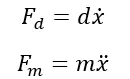
The sum of all forces acting in a different direction is given as follows,

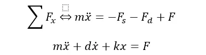
This is the equation of motion (EoM) and it is in the form of 2^nd order ordinary differential equation (ODE), linear in nature, with constant coefficients and inhomogeneous.

The above equation was in the differential form we can convert it into the s domain or frequency domain which is represented as follows,

Finally, we can rearrange the equation to get the transfer function G(s) of this system. The definition of the transfer function of a control system is its outputs divided by its inputs. In this case, X(s) is the output, F(s) is the input, so we can get G(s) as follows:

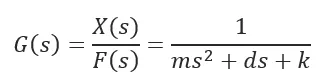
The above-derived ODE can be converted to a single-order equation by using a state-space representation of the mass-spring-damper system. The Laplace transformation ignores the initial condition of the system.

A PID controller has some limitations also apart from being one of the best controllers in the control action system. PID control is applicable to many control actions but it does not perform well in the case of optimal control. The main disadvantage is the feedback path. PID is not provided with any model of the process. Other drawbacks are that PID is a linear system and the derivative part is noise sensitive. A small amount of noise can cause great change in the output.

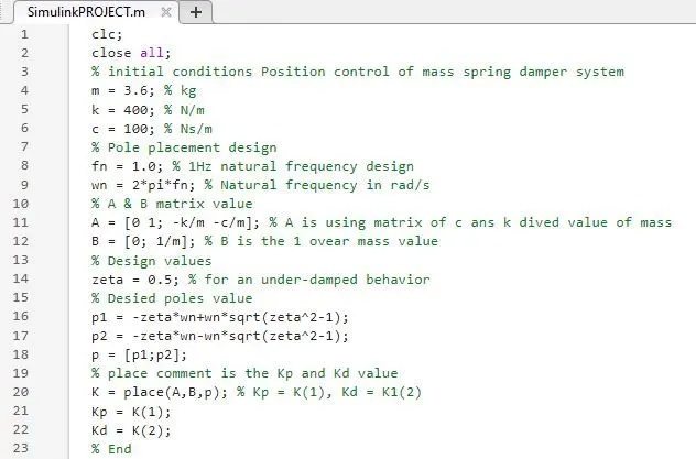
To control the displaced position of the mass after the force acting on it, we have to use a PID controller. Here zeta value=1.001(critically damped condition) is considered by using zeta value Poles(P1, P2) are calculated and then Calculate kp (Proportionality constant), Kd (differential constant) by using the place command. Ki value is manually modified to control the output wrt input.

Here the input is a pulse-generated signal with an amplitude of 1 and a period of 10. as given in the question.

The script file written to find the poles, kd, and kp values is below.

The simulink model is built based on the transfer function equation. and PID controller is added before the plant transfer function. Pass the m, c, k, kp and kd values to the model blocks and change the ki values from 0 and observe the output wrt input.

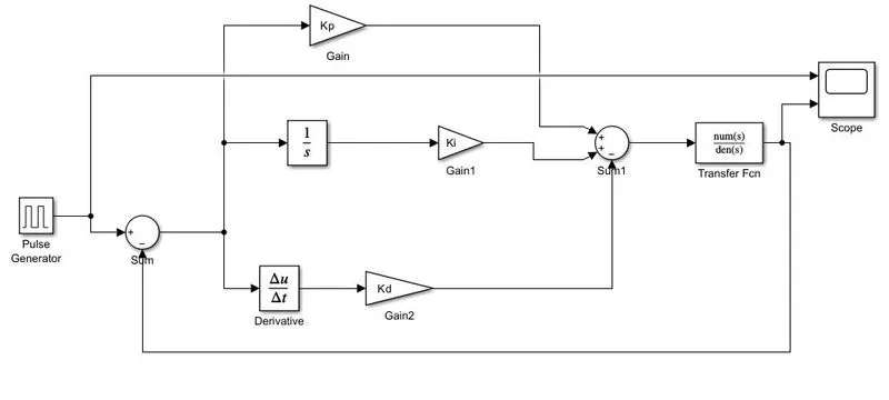
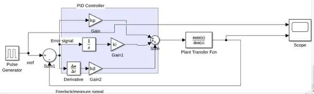
Here error signal is generated by taking the feedback output and given to the comparator to compare with the reference signal(Pulse generator) each time then gives the output to the PID controller, and the PID controller output is given to Plant(Spring mass damper) transfer function. Like this, the output is rectified with an error changing the values of ki manually.

The first value of ki is taken as ki=0;

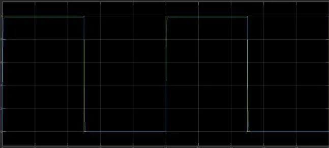
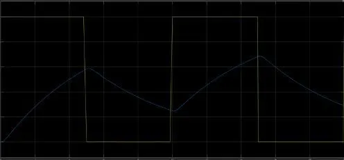
when Ki = 0, we can observe that there is a steady state error between the reference and simulated signal.

• The input reference signal is input through the system by using a Pulse generator having an amplitude of 1 and a period of 10 seconds.
• The transfer function of the Spring mass damper system is implemented in the system by using the Transfer function.
• The input for the Integral gain Ki is fed through the integrator block and reference signal output. The initial response of the Ki was set to zero to record the response with the reference signal.
• The PID gains such as Kp and Kd values are calculated by running a Matlab file and subsequently updating those values in the system.
• By running the place command placement of the pole is calculated.
• If we used the derivative block with the proportional gain to compare the output results. As we got a steady state error which was an overlapping overshoot response.
• To compensate for the above error we have introduced a demux block to output separate signals coming from Kp and Ki gains.

Setting Ki as 50

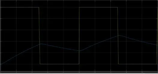
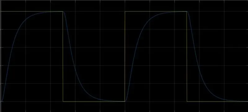
As we can see from the above plot we can observe that rise time and settling time is decreasing.

Increasing Ki value to 100

Conclusion:

To complete the project of Position control of mass spring damper system transfer function of a mass spring damper system and use it in the model. Add a PID controller to adjust the force on mass so that its position follows a reference signal using matlab and simulink wave from the plot.

The Matlab Script file and Simulink model file are attached here.

https://drive.google.com/file/d/1zYLDZJQhdmL2reO_hAU8m3X9G_dtSfjS/view?usp=share_link

https://drive.google.com/file/d/1ck1wTxoFnIvQbzzivnh6PIvOLdMOTcVC/view?usp=share_link