Project - Position control of mass spring damper system

Q1) .Obtain the transfer function of a mass spring damper system and use it in the model. Add a PID controller to adjust the force on mass so that its position follows a reference signal.

Take m = 3.6; %kg k = 400; %N/m c = 100; %Ns/m

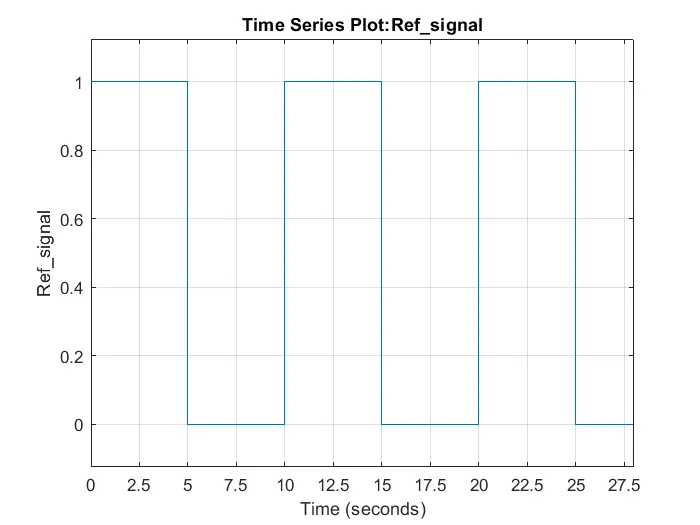
The reference signal is shown in the following figure.

Project - Position control of mass spring damper system

Diagram of spring Mass Damper system:

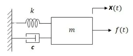
Where, f(t) = external force applied on mass

x(t) = Displacement / Position

m = mass

k = spring constant

c = damping coefficient

Newton’s second law states that an applied force is proportional to the rate of change of momentum

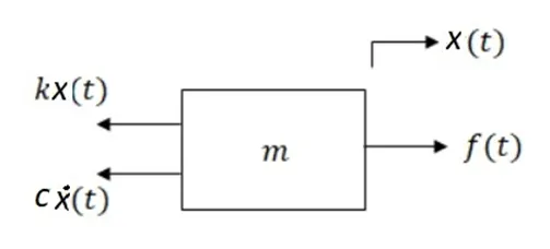
Mathematically,

F = ma; F = m*d(v)/dt

If x represent the displacement, x. represent the velocity, x.. represents the acceleration, then the equation ca be written as

F = ma, = m*xdot_dot

Here the dot represents the time derivative.

the governing equation can be written as

F(t) = m*x.. + c*x. + k*x

Where c is the damping coefficient and k is the spring stiffness constant

Both F and x are the function of time.

Differential equation in the form to represent the mechanical system that are termed as ‘Spring-Mass-Damper’ systems.

F(t) – c *dx/dt – k*x(t) = m*d^x/ dt^2 ------------------equ (1)

In Matlab and Simulink, the differential equations are converted into algebraic equations by using the Laplace transform.

The Laplace transform of a function F(t) is equation no 1 written as;

F(s) - cs*X(s) - k*X(s) = ms^2*X(s)

X(s) / F (s) = 1/ (m*s^2 + c*s + k)

X(s) / F (s) = 1/ m / [(s^2 + c/m*s + k/m)] -----------------Divide by m to Numerator and Denominator.

Block Diagram:

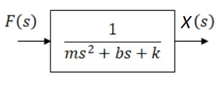
It is easier to simplify the transfer function using the Diagram to arrive at a combined transfer function with a numerator and denominator polynomial in the Laplace Variable , ‘s’.

The requirement is that the combined transfer function is a rational transfer function with order of numerator polynomial being at least one degree lower than Denominator.

The combined transfer function can be split into individual function using a well-known method called ‘partial Fraction Expansion’.

State vector:

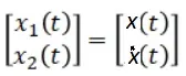
Input vector

[u(t)] = [f(t)]

Output vector

[ y(t)] = [x(t)]

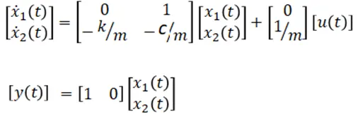
Rewrite equation

u(t) – c*x2(t) – k*x1(t) = m*x2dot(t)

Rearrange equation to xdot(t) and y(t) in terms of x(t) and u(t)

x1dot(t) = x2(t)

x2dot(t) = -k/m*x1 – c/m * x2(t) + 1/m* u(t)

y(t) = x1(t)

Organize in matrix format:

Xdot = A*X + B u

Now we have to write State Space Model for that we have to find A and B Matrix.

The Control of Spring Mass damper Model used Simulink Blocks are below:

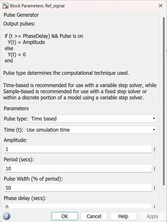
Pulse Generator

The Pulse Generator block generates square wave pulses at regular intervals of time. The block waveform parameters, Amplitude, Pulse Width, Period, and Phase delay, determine the shape of the output waveform.

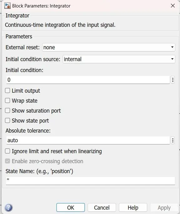
Integerator

The Integrator block outputs the value of the integral of its input signal with respect to time.

Simulink treats the Integrator block as a dynamic system with one state

˙x(t) = x(t)

y(t) = u(t)

x(t0) = x0

where:

Derivative

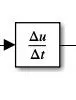
The Derivative block approximates the derivative of the input signal u with respect to the simulation time t. You obtain the approximation of

by computing a numerical difference Δu/Δt,where Δu is the change in input value and Δt is the change in time since the previous simulation (major) time step.

This block accepts one input and generates one output.

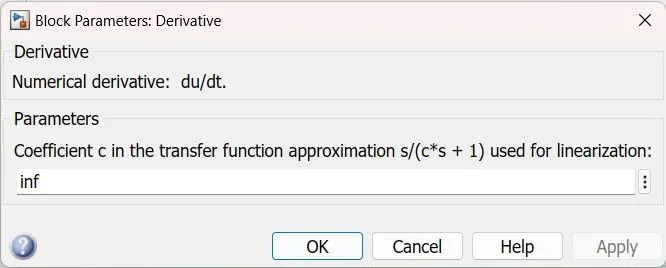
Gain

The Gain block multiplies the input by a constant value (gain). You specify the value of gain in the Gain parameter

Summing junction

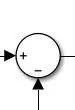
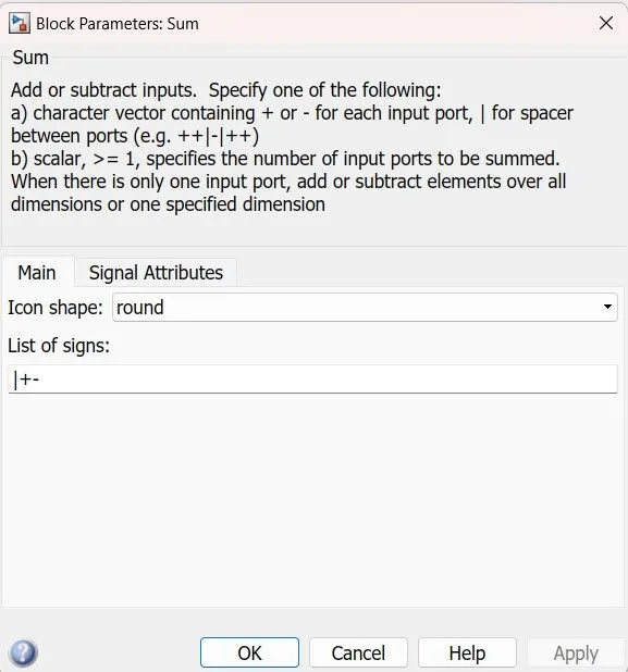
The Sum block performs addition or subtraction on its inputs.

character vector containing + or - for each input port.

Transfer function

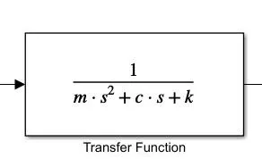
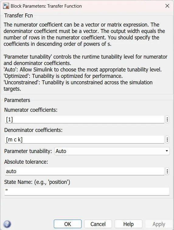
In the Transfer function block, numerator coefficient can be a vector or matrix expression, But the denominator coefficient must be a vector.

The output width equals the number of rows in the numerator coefficient. You should specify the coefficients in descending order of powers of s.

Scope

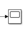
Display signals generated during simulation with respect to time. we can connect n numberof input.

Simulink Block Diagram of control on Spring Mass Damper

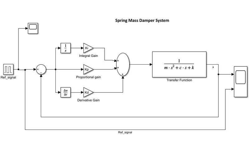
A PID Controller stands for proportional-integral-Derivative is a control loop mechanism feedback. PID is widely used in industrial control system.

the given reference signal we assign in the Pulse generator, Amplitude=1, Period= 10, pulse width= 50; in this for 5 sec system will ON and another 5 sec OFF. whatever refeence signal comming from pulse generator is applied to on of the port of summing junction. Substract the reference speed to the error signal e(t).

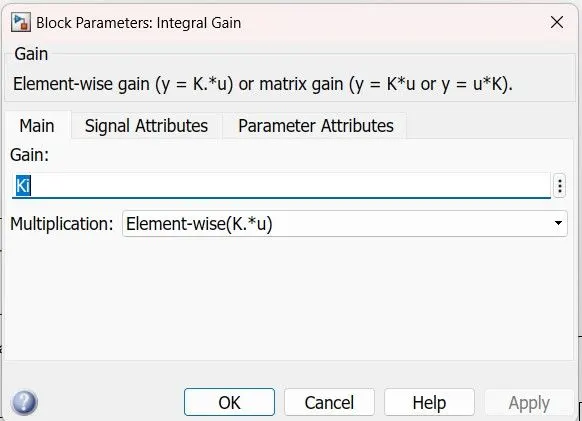
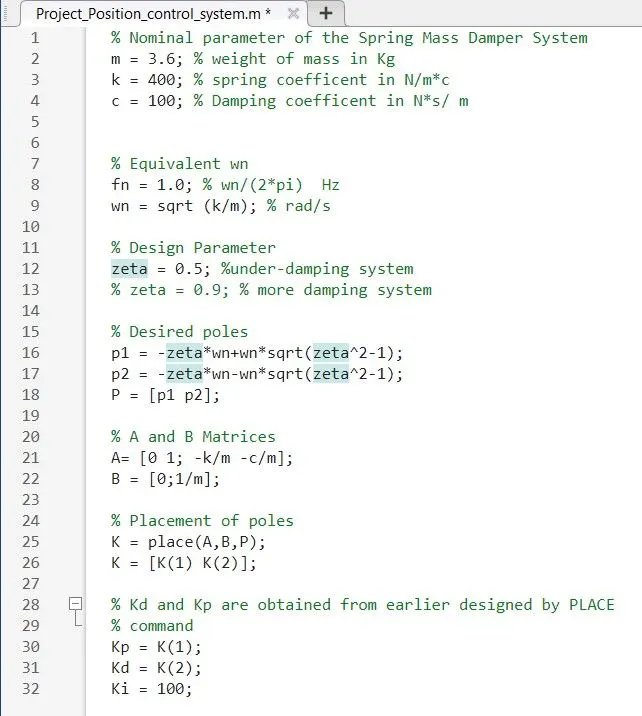
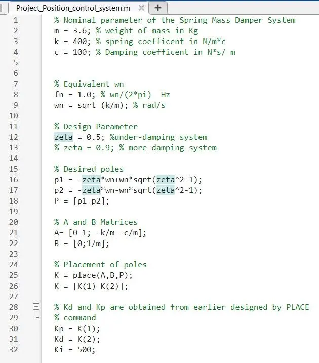
Add Kp as K(1) and Kd as K(2) parameter determined from place command (K=place(A,B,P)). use gain block to mention values of Kp, Kd, and Ki.

Add Ki manually with gain and integrator block and tune different values of Ki and check the values of Ki.

When there is a mass in a system, its position and velocity are commonly chosen as state variables. Also, position, velocity, and force (input) are sufficient to determine this system's future position (output). For these reasons, position and velocity are chosen as state variables.

Here given parameter are m = 3.6; %kg k = 400; %N/m c = 100; %Ns/m.

Matlab Code:

zeta = 0.5 which is under damper system, Ki = 100

In place of scope result we taken a Data inspector result:

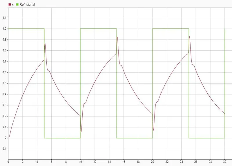
Here we can see our system position output signal gradually increase but not follows 0 to 5 sec .

There is a more gap between the response signal and our reference signal it is known as steady state error.

case-2

zeta = 0.5 which is under damper system, Ki = 200

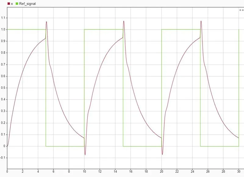
Here we can see our system position output signal gradually increase but not follows 0 to 5 sec .

There is a less gap between the response signal and our reference signal compare to earlier case it is known as steady state error.

case-3

zeta = 0.5 which is under damper system, Ki = 400

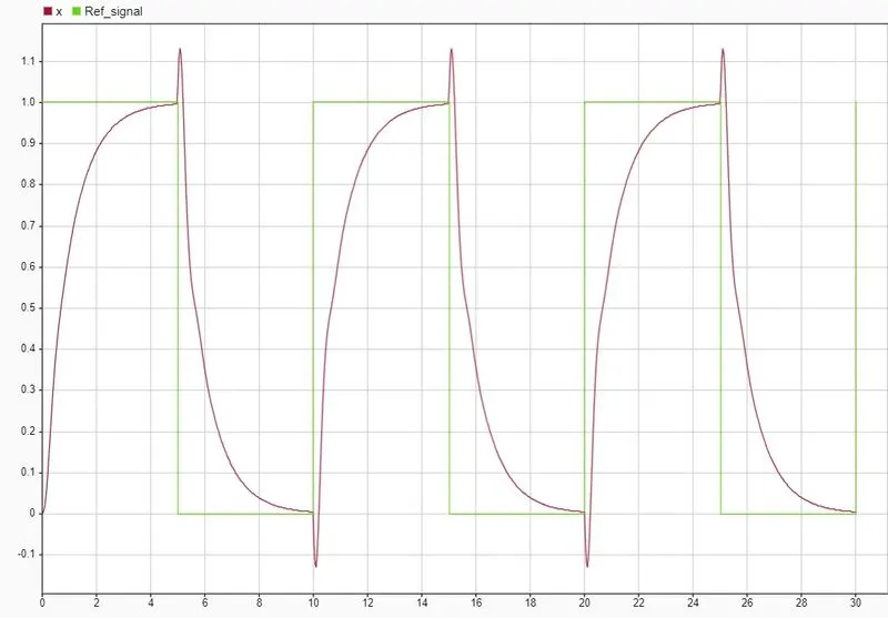
Here we can see our system response gradually increase setteling at 5 sec.

There is a no gap between the response signal and our reference signal it has no steady state error.

case-4

here increase to Ki= 500 ; zeta-= 0.5

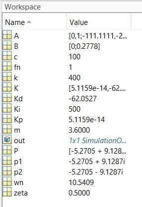
Workspace Variable:

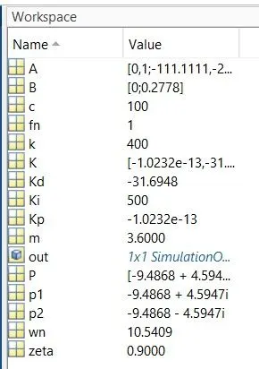
we can find value of zeta, Ki, KP,Kd

Data inspector Result:

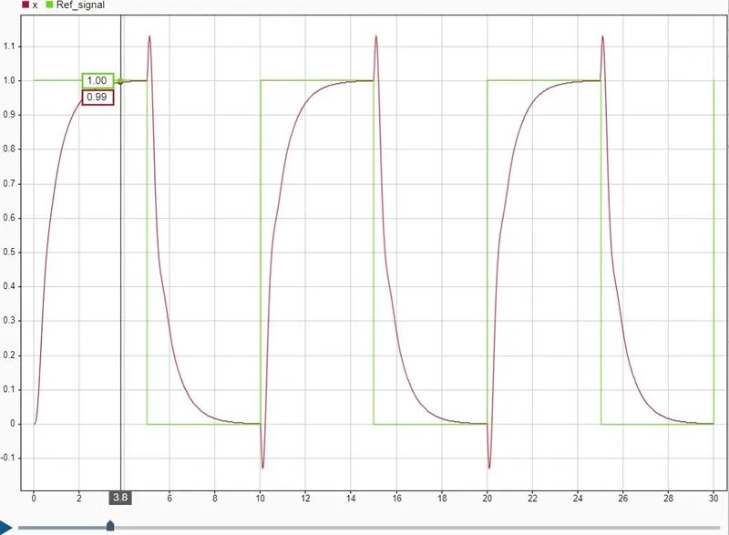
here zeta = 0.5 and integral gain Ki = 500, our response starts from its initial position. the response settle after 3.8 second.

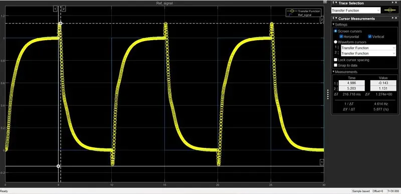
in this scope result time period 4.99 to 5.20 sec aproximately 0.21 sec overshoot occur and 5 sec to 10 sec, the response continously fall down and negative oveshoot is also occur.

case - 5

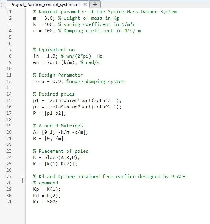
Now in this case we increase the damping from 0.5 to 0.9

Matlab Code:

Workscape Variable:

Data inspector Result:

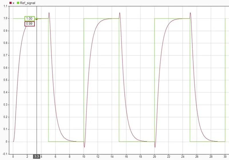
here, zeta = 0.9 and integral gain Ki = 500, our response starts from its initial position. the response settle after 3.3 second

Conclusion :

• we Obtained the transfer function of a mass spring damper system and use it in the model.
• Added a PID controller to adjust the force on mass so that its position follows a reference signal.

where m = 3.6; %kg k = 400; %N/m c = 100; %Ns/m

• we set the parameter in The reference signal is shown in the following figure into the Pulse Generator.

• when zeta = 0.5 and Ki = 500, response take to more time to settle or follow but when zeta = 0.9 and Ki = 500 kept same, compare to earlier it follows before or settling time take less.

Reference:

https://cookierobotics.com/008/