Project

Carry out a system-level simulation of an all-terrain vehicle.

Download the model from the given link:

https://www.mathworks.com/matlabcentral/fileexchange/70576-baja-all-terrain-vehicle-atv-model

Prepare a technical report explaining the model properties & comments on the results.

Module (1): PROJECT

Aim: To Prepare a Technical Report on Modelling of a Continously Variable Trainsmission for BAJA All-Terrain Vechile Model.

Summary:

ABOUT THE MODELS- These models show how to build an ATV with CVT which is mostly used in BAJA competitions. Simscape and Simscape Driveline have been used to complete the system. The engine data used in the model is provided as an image which shows the Engine Speed (RPM) Vs Torque curve.

Team Synergy of G.L. Bajaj Institute of Technology and Management, who give images, Event and Specification of the Baja Vehicle.

Introduction:

It contains a set of various Tools to created this model with;

• MATLAB
• Simulink
• Simscape
• Simscape Driveline

BAJA ATV

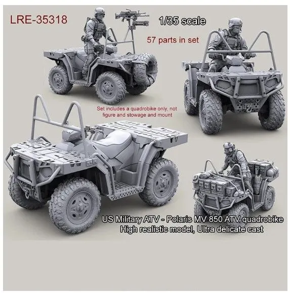
• An All-terrain vehicle (ATV), also known as a light utility vehicle (LUV), a quad bike, or simply a quad, as defined by the American National Standards Institute (ANSI); is a vehicle that travels on low-pressure tires, with a seat that is straddled by the operator, along with handlebars for steering control. As the name implies, it is designed to handle a wider variety of terrain than most other vehicles. Although it is a street-legal vehicle in some countries, it is not street-legal within most states, territories and provinces of Australia, the United States or Canada.
• By the current ANSI definition, ATVs are intended for use by a single operator, although some companies have developed ATVs intended for use by the operator and one passenger. These ATVs are referred to as tandem ATVs.
• The rider sits on and operates these vehicles like a motorcycle, but the extra wheels give more stability at slower speeds. Although most are equipped with three or four wheels, six-wheel models exists and existed historically for specialized applications. Multiple-user analogues with side-by-side seating are called utility terrain vehicles (UTVs) or side-by-sides to distinguish the classes of vehicle. Both classes tend to have similar powertrain parts

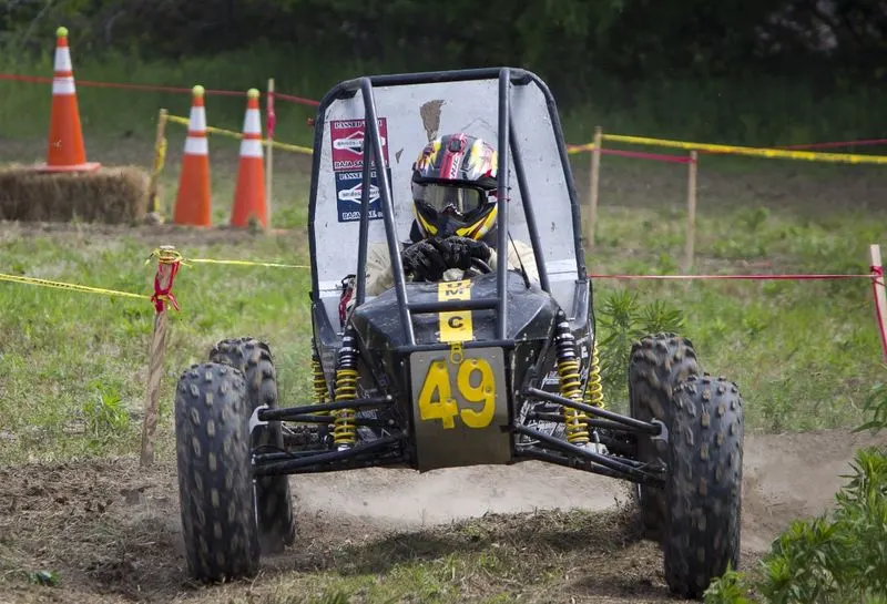
BAJA SAE:

• Baja SAE is an Collegiate Design Series competition run by the Society of Automotive Engineers International (SAE International). Teams of students from universities all over the world design and build small off-road cars. The cars all have engines of the same specifications. As of 2018 the engine has been an unmodified Briggs & Stratton Model 19 Vanguard engine single-cylinder with a displacement of 305cc and power output of approximately 10 bhp (7.5 kW).
• The goal in Baja SAE racing is to design, build and race off-road vehicles that can withstand the harshest elements of rough terrain. The vehicles used in Baja SAE racing are often similar in appearance to dune buggies. Before 2007, the events were called "Mini Baja."

1) Component of BAJA ATV:

a) CVT ( Continuously Variable Transmission)

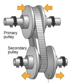
A Continuously variable transmission (CVT) is an automatic transmission that can change seamlessly through a continuous range of gear ratios. This contrasts with other transmissions that provide a limited number of gear ratios in fixed steps. The flexibility of a CVT with suitable control may allow the engine to operate at a constant RPM while the vehicle moves at varying speeds.

CVTs are used in automobiles, tractors, motor scooters, snowmobiles, bicycles and earthmoving equipment.

The most common type of CVT uses two pulleys connected by a belt or chain; however, several other designs have also been used at times.

Simulink ATV Model

• BATA ATV Model-CTV Model (without Dashboard)

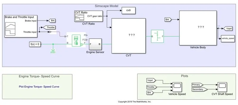
In the above given model the simulink Blocks are used as follows:

1) Signal Builder: The Signal Builder block allows you to create interchangeable groups of piecewise linear signal sources and use them in our model.

2) Simulink-PS Converter: The Converter use to convert Simulink input signal into Respective Physical Signal.

3) Solver Configuration: The solver configuration specifies the solver parameters that your model needs before you can begin Simulation. Simscape Block diagram require exactly one solver configuration block to be connected to it.

7) Go To: The Goto block passes its input to its corresponding From blocks. The input can be a real- or complex-valued signal or vector of any data type. From and Goto blocks allow you to pass a signal from one block to another without actually connecting them.

8) From To: The From block accepts a signal from a corresponding Goto block, then passes it as output. The data type of the output is the same as that of the input from the Goto block. From and Goto blocks allow you to pass a signal from one block to another without actually connecting them

9) Scope: Display signals gererated During simulation.

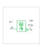
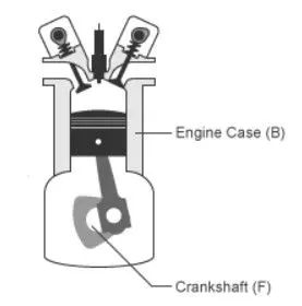
4) Generic Engine: This block Represents a system-level model of spark-ignition and diesel engines

5) Engine Sensor: It is a Subsystem of model consists of the following given Simulink block Below:-

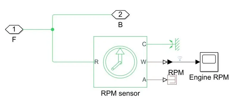Ideal Rotational Motion Sensor: The Ideal Rotational Motion Sensor block represents an ideal mechanical rotational motion sensor, that is, a device that converts an across variable measured between two mechanical rotational nodes into a control signal proportional to angular velocity or angle.

Mechanical Rotational Reference: This block represents a Reference point or frame, for all Mechanical Rotational port.

PS-Terminator: Use this block to terminate physical signal outputs.

PMC-Port: Physical Modeling Connection Port block for subsystems.

Scope: Display signals gererated During simulation.

PS-Simulink converter: It convert the input physical signal to Simulink output signal.

6) Simple Gear: The Simple Gear block represents a gearbox that constrains the connected driveline axes.

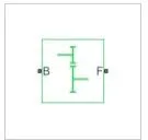
B= the base gear,

F= the follower gear,

to corotate with a fixed ratio that you specify.

CVT: It is a Subsystem Model consists of the following simulation blocks:

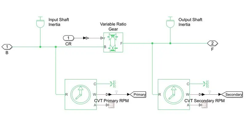
Inertia: This block Represent an ideal Mechanical Rotational inertia.

Import: Inport blocks link signals from outside a system into the system.

Ideal Rotational Motion Sensor: The Ideal Rotational Motion Sensor block represents an ideal mechanical rotational motion sensor, that is, a device that converts an across variable measured between two mechanical rotational nodes into a control signal proportional to angular velocity or angle.

Variable Ratio Gear: This block Represents a variable ratio gearbox such as implemented by mechanical belt CVT, electric, or hydraulic transmissions. The physical signal input r defines the ratio of input to output angular shaft velocities.

Mechanical Rotational Reference: This block represents a Reference point or frame, for all Mechanical Rotational port.

PS-Terminator: Use this block to terminate physical signal outputs.

PMC-Port: Physical Modeling Connection Port block for subsystems.

Go To: The Goto block passes its input to its corresponding From blocks. The input can be a real- or complex-valued signal or vector of any data type. From and Goto blocks allow you to pass a signal from one block to another without actually connecting them.

PS-Simulink converter: It convert the input physical signal to Simulink output signal.

Simple Gear: It Represent fixed gear ratio or Gear Box.

Vehicle Body: It is a Subsystem model consists of the following Simulation Blocks:

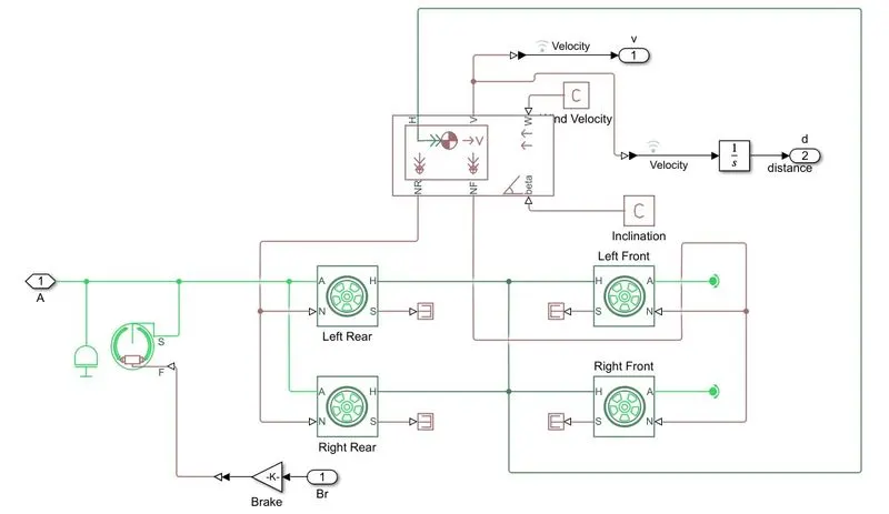
Inertia: This block Represent an ideal Mechanical Rotational inertia.

PMC-Port: Physical Modeling Connection Port block for subsystems.

Double Brake Shoe:

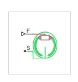
The Double Brake shoe block Represents a brake arranged as two pivoted rigid shoes symmetrically installed inside or outside a drum to produce a braking action and operated by one actuator. The actuator force causes the shoes to exert a friction torque on a shaft connected to the drum.

Gain: The Gain block multiplies the input by a constant value (gain).

Element-wise gain (y = K.*u) or matrix gain (y = K*u or y = u*K).

Tire:

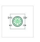
• Connection A= the mechanical rotational conserving port for the wheel axle.
• Connection H= the mechanical translational conserving port for the wheel hub through which the thrust developed by the tire is applied to the vehicle.
• Connection N= a physical signal input port that applies the normal force acting on the tire. The force is considered positive if it acts downwards.
• Connection S = a physical signal output port that reports the tire slip

PS-Terminator: Use this block to terminate physical signal outputs.

PS-Constant: This block creates a physical signal constant.

Integrator: The Integrator block outputs the value of the integral of its input signal with respect to time.

PS-Simulink converter: It convert the input physical signal to Simulink output signal.

Simulink-PS converter: It convert the input physical signal to Simulink output signal.

2) Vechile Modelling:

a) Open Loop

BAJA ATV MODEL without Dashboard

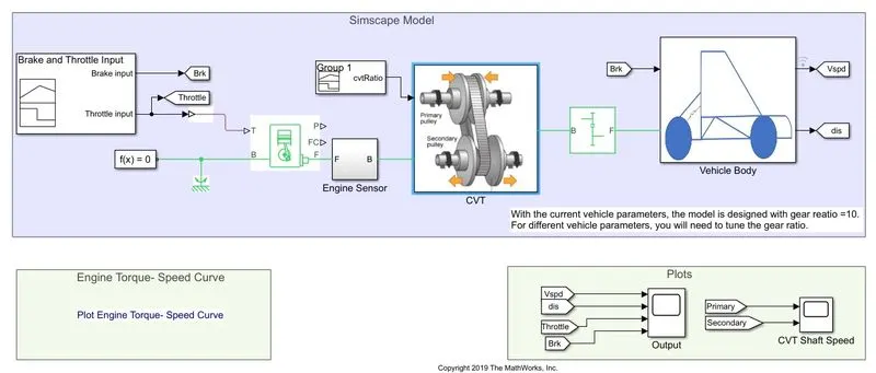
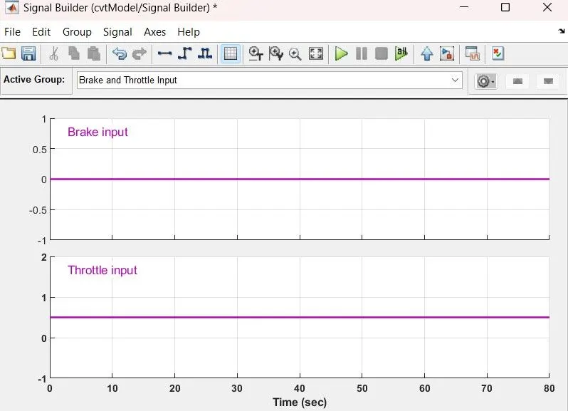
i) By Using Signal Builder we are giving brake and Throttle Input to Generic Engine.

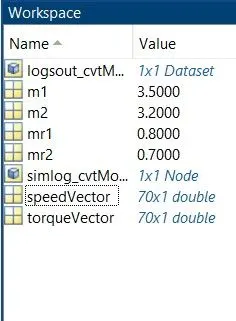
a) The Variables m1 and m2 stand for the Mass input of the Input shaft and Out shaft at CVT Transmission system.

b) The Variables SpeedVector and TorqueVector are the Engine Parameter of the Generic Engine, which provide the Relationship between Torque and RPM of the Engine.

c) We have in the Inital condition of the generic engine block is set according to the engine parameters, and then according to the Throttle input input changes its Parameter of Speed and Torque. In this Model the Engine Parameters Provide through Workspace by create Variables (SpeedVector and TorqueVector).

d) After getting the Throttle input it provide the RPM, Torque, and various factors depending on the Generic Engine Parameters.

e) The Output of the Generic Engine give to Engine Sensor block, the Sensor will measure the RPM of the Engine During Simulation and then forward toward the CVT System.

f) The CVT block is a Subsystem, it has two input one from Engine Sensor and another from Signal Builder which is provide by CVT Ratio.

g) In the CVT block, there are two Ideal Rotational Motion Sensor and two inertia Blocks for both Input and Output shaft respectively, and there is a Variable Gear Transmission block is there which can changes its gear ratio according to CVT Ratio where the gear ratio.

h) After getting the input signal, it passes to Simple Gear block which we can say that it is Act as Differential Gear Box before passing to the Vehicle Body.

i) In the Vehicle body there is a two inputs one from the Simple Gear and another from the Brake input.

j) since our model is design on the basis of aTWD (Two Wheel Drive), Vehicle the input engine signal from the simple gear is provide to both Rear Wheel of vehicle body.

k) there is a Rotational input inertia is connected to shaft so it is connected to the engine input signal before it reaching to the Tire.

l) The other input Brake is provided to the Double shoe Brake Block, but Before it reaches it passes through Gain block in other words it is act as Brake input, it Multiples input force to the Gain factor is 1000.

m) As the Brakes are indirectly to the input Power of the wheels, hence the out from the Double shoe Brake Block is connected to the Engine input signal before it reaching to Tire.

n) Here there is a another Vehicle Body (inside the Vehicle Body of the System) The block accounts for body mass, aerodynamic drag, road incline, and weight distribution between axles due to acceleration and road profile, with the help of vehicle dynamic Data provided to the block it Distrubute on the Normal Forces on the Tire.

o) we also get the Velocity of the Vehicle as in output from the Vehicle body block.

p) As the Velocity signal passes through Integrator block, and it provide the Distance covered by the Vehicle.

q) We have the results of the Simulation if three scope Data, in which one from the Engine RPM, second from the RPM of the Primary and Secondary shaft CVT system and the third from Velocity, distance, Throttle and Brake values of the Vehicle.

I) Here, the result Simulation for 200sec.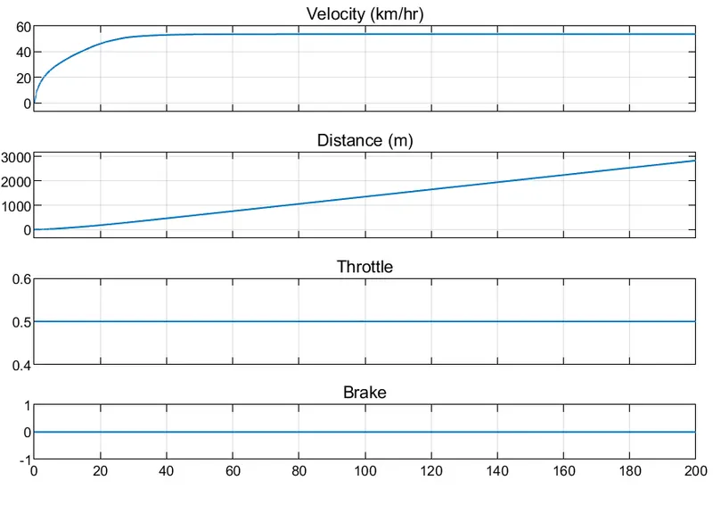

a) Here, we can see that the Throttle and Brake value inputs are constant during the complete Simulation.

b) The Velocity of the Vehicle is gradually increase and After a certain ponit when the engine reaches it constant RPM, the velocity of the vehicle become constant.

c) As we know integration of the velocity give us Distance travel by the Vehicle. Hence during the Simulation initial time, the distance travelled by vehicle it looks like aparabolic curve, and when the velocity of the vehicle become constant then the distance travelled by vehicle become straight line.

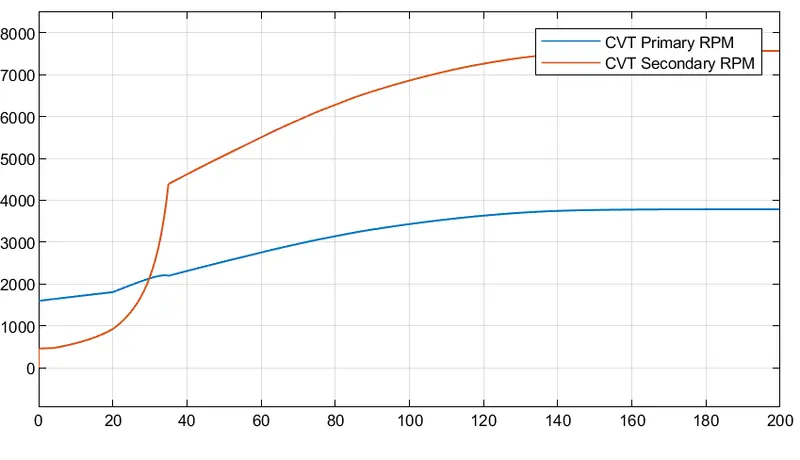
II) Result of CVT shaft speed:

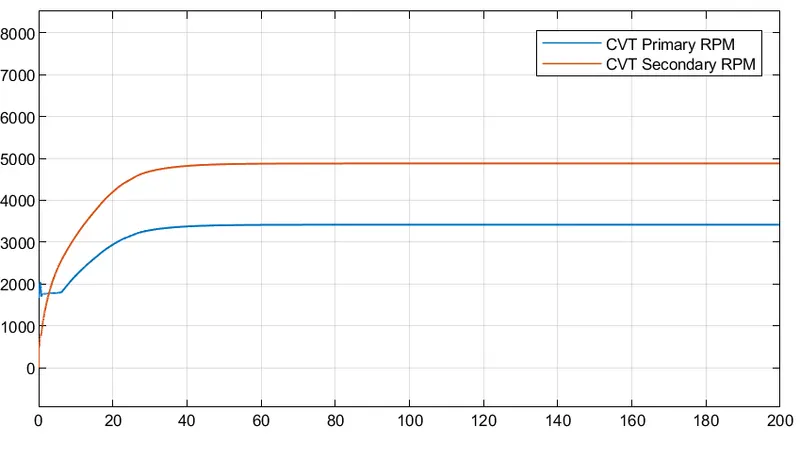
In the above Graph, the CVT Primary RPM is slightly increase from some instant of time (3 to 10 sec) and after that it gradually increase (10 to 40 sec) and after it remains constant from 40sec.

In this case, the RPM of CVT Secondary shaft look like same as that of velocity of the Vehicle above.

In this case Brake input=0, Throttle input=0.3

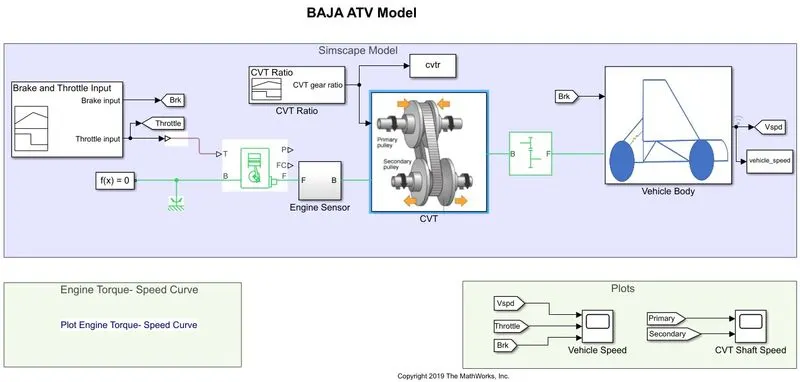
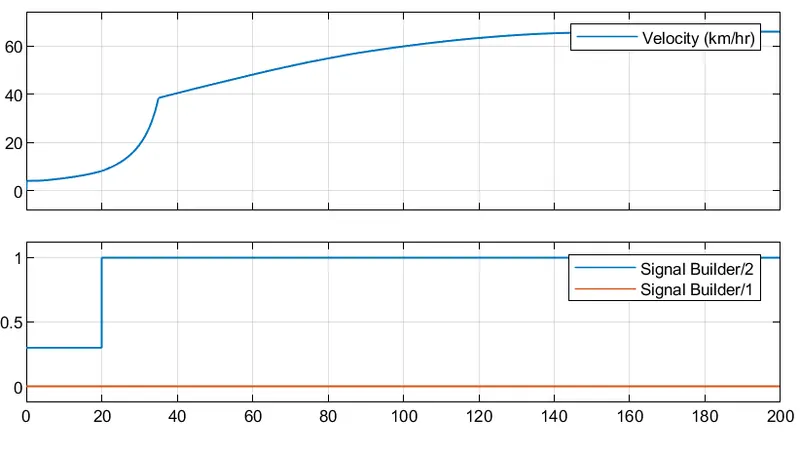
a) Here, we can see that the Throttle signal is generated by signal builder block and fed input to the Generic Engine and Brake value input is constant during the complete Simulation.

b) The Torque vector and speed vector are inputted from the Matlab Workspace.

c) From this graph, we can refer that the brake is not applied during the cycle and the throttle is constant (0.3) upto 20 sec and being increased from 0.3 to 1 at 20sec where it is remain constant for the rest of the Time with the increase in Throttle input, the vehicle speed is also increase.

d) The Velocity of the Vehicle is gradually increase and After a certain ponit when the engine reaches it constant RPM, the velocity of the vehicle become constant.

The Generic Engine will Generate the output RPM which can be taken from Crankshaft output.

The speed will be given to Ideal Rotational Motion sensor to sense the output RPM

The same output will be giving to Simple Gear Mechanism to Reduce the speed where Gear Ratio kept '4'.

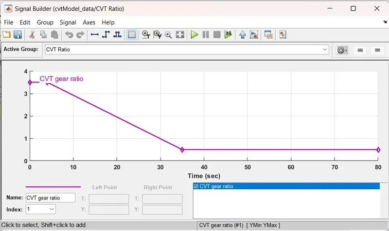
The CVT Ratio is Provided to Variable Gear Ratio Transmission (CVT) block through signal builder.

The speed is controlled by variable CVT Ratio and controlled output speed is inputted to the Vehicle Axle.

The brake signal is provided from signal builder block and inputted to Vehicle boby (i.e. Doubble Brake shoe) for applying the Brake to the Axle.

The Power from the CVT is inputted to the Axle and the Vehicle is accelerates according to the speed.

Then the Velocity is taken as output from the Vehicle Body for futher analysis.

BAJA ATV Model 1 with Dashboard

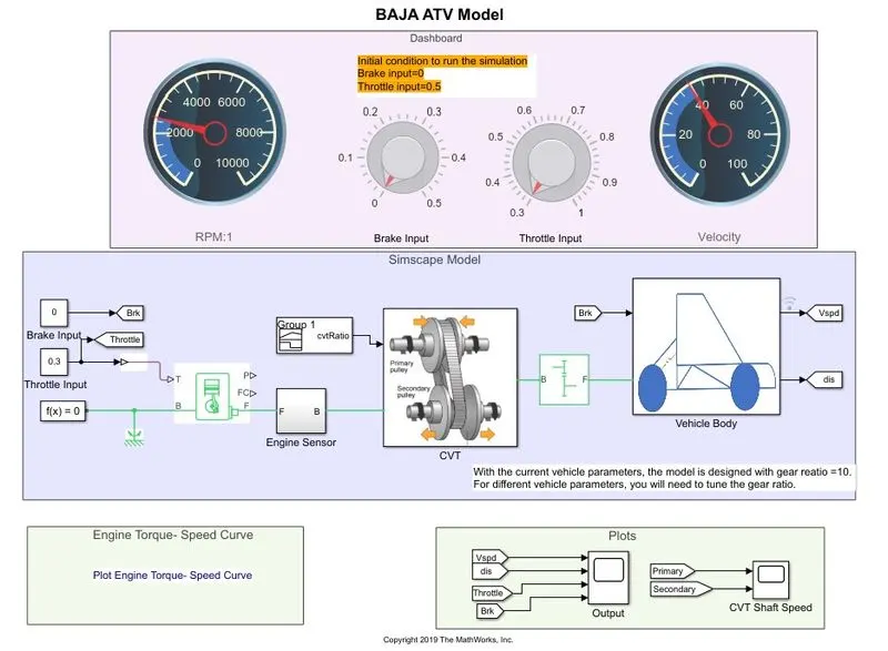
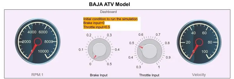
Workflow:

i) Here, the Model is same but there is that in place of Signal Builder, replace with knob for Throttle and Brake inputs and also using constant Block.

ii) we can change the value of Throttle and Apply the Brake input by knob, will change in Velocity and RPM of the Vehicle that can be Observe also.

iii) The above show circular guage it display an input on a Customize Gauge.

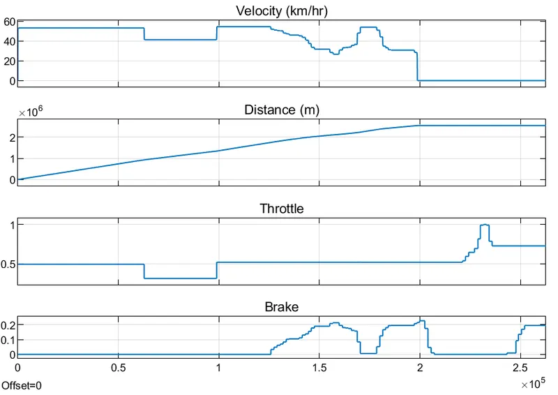
i) At initial condition to run the simulation brake input=0 and throttle input=0.5 this is given

ii) After 0.5sec brake value input kept zero remains constant, but the throttle value put to 0.5 to 0.3 upto 1 sec

iii) Distance travel by the Vehicle increase gradually and After a certain ponit when the engine reaches it constant RPM, the engine speed of the vehicle become constant

iv) The Velocity of the Vehicle is already high 53.33km/hr upto 0.6sec but it is same like that of throttle input values and after that it is constant for certain ponit.

v) when we apply brake input value slightly increases that will change to velocity of the vehicle decreases.

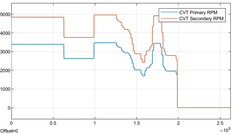
i) here, from the above graph we can observe that in CVT Transmission system of vehicle the Primary RPM and Secondary RPM as like both are same as throttle input and velocity of the vechile.

ii) when we apply brake the Primary RPM and Secondary RPM of the vehicle get reduce the speed.

b) Close Loop

BAJA ATV Model with Dashboard (Mapped Lookup)

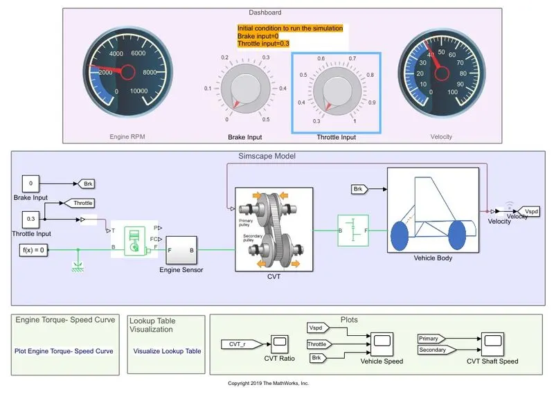
Workflow:

i) Here, the Model is same but there is that in place of Signal Builder, replace with knob for Throttle and Brake inputs and also using constant Block.

ii) we can change the value of Throttle and Apply the Brake input by knob, will change in Velocity and RPM of the Vehicle that can be Observe also.

iii) The above show circular guage it display an input on a Customize Gauge.

iv) It is a close loop type Model, which the output of Velocity if the vehicle given to input of Lookup Table Block.

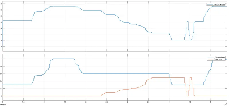
Here Throttle input= 0.3, brake input=0

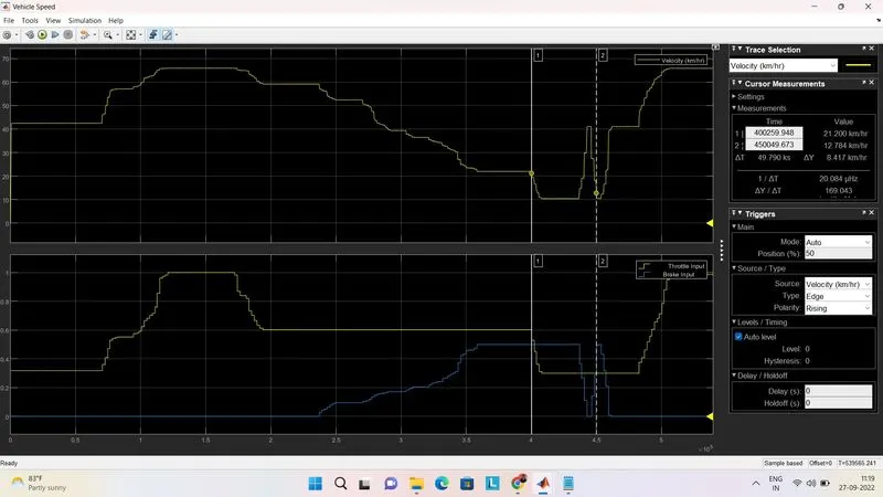
In this case:

i) when brake input=0 upto 2.2 sec, but Throttle input =0 upto 0.7 sec, at this instant the Velocity of the vehicle Run at its constants Speed.

ii) After that we can Throttle input increase slightly with the help of Knob from 0.3 to 1. at Brake input still=0, at this instant the Velocity of the vehicle Run its Maximum Speed from (43 to 65) km/hr and Vehicle run its constnt speed upto wheneever brake is not appllied.

iii) Throttle input= 0.6 and brake input= 0.5 at time= 4sec in this instant velocity of the vehicle= 21 km/hr and after certain time that throttle input slightly decrease to 0.3 where brake input kept= 0.5, at this instant Velocity of the vehicle Reduce the speed.

iv) Throttle input= 0.3 and Brake input= 4.9 at time= 4.5sec in this instant velocity of the Vehicle= 10 km/hr

v) Throttle input= 0.3 where brake input kept= 0, at this instant Velocity of the vehicle= 41 km/hr it increase the speed.

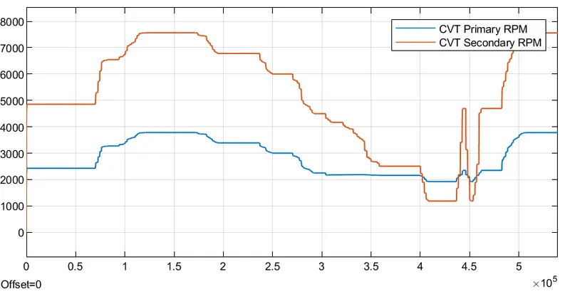
• With the help of above graph initally Primary CVT = 2430Rpm and Secondary CVT = 4860Rpm constant upto at 0.7 sec, at this instant Throttle input=0.3 and Brake input=0 and also speed of the Vehicle= 43 km/hr.
• After certain of time Primary CVT = 3780Rpm and Secondary CVT = 7570 Rpm constant upto at 1.5 sec, at this instant Throttle input=0.3 and Brake input=0 and also speed of the Vehicle= 43 km/hr.
• As the Primary shaft is connected to Engine the Behaviour of both Primary and Secondary CVT it is similar to Engine RPM
• Whatever output from the CVT it is feding to Vehicle Body and it is giving to Axle of the wheel which the bechile ot moving.

• Whatever looking here it is inside of the Model, which is kwon as subsystem of CVT:

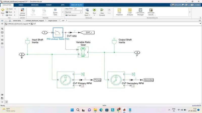
i) Here we use instead of signal Builder for CVT Ratio input to Variable Gear, 1-D lookup Table Block is used.

ii) This block represents a physical signal converter whose input-output relationship is specified by a lookup table. The table grid must be in strictly ascending or strictly descending order, but the spacing can be nonuniform.

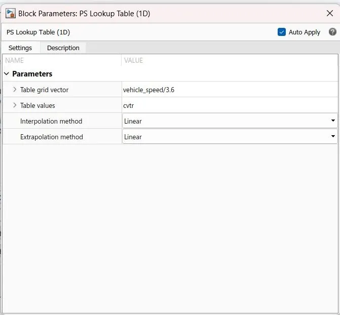
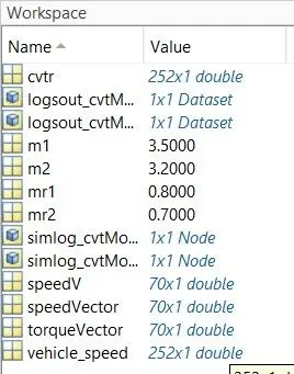
• We can get the Vehicle Speed which is fed into Matlab Workspace through Variable as cvtr.

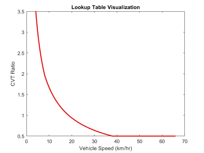
• Right-click on the block and select Foundation Library > Plot Table to visualize the table data based on the selected interpolation and extrapolation methods as follows:
• That show the Relationship Between CVT Ratio and Velocity Below:
• In this graph velocity gradually Decrease with the increase of given CVT Ratio value.

3) Incorporating CVT data into the Model:

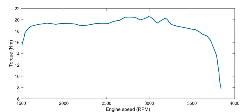
• In this Model the show graph Torque and Engine speed values not Provided.
• For taking this values form the workspace, we have to download we can use in 'File Exchange' search "GRABIT".
• with the help of this app we can Extract those Data points.
• It Means that we can easily convert the image file into Data points values and that can be fed in the Generic

Engine.

• The Maximum Speed of the Baha Engine is 3840RPM, when the Torque is 8(Nm) and the the Engine will stop.

Conclusion:

• With this Model it help us to verify the performance of the Vehicle given Brake and Throttle Inputs.
• We observe that what will be the maximum speed of the Vehicle can achive by Defining the Gear Ratio.
• With this Model we can understand how Vehicle perform under the Given different Models.
• We can control to the Model with the help of Given Dashboard Knob.
• Use sufficent Realistic data into model Real-World condition.