Project - Position control of mass spring damper system

Position control of spring mass damper system:

Given datas:

m=3.6 kg

k=400 N/m

c=100 Ns/m

Transfer function of spring mass damper system

f(t)-cdx/dt-kx=m*d^2x/dt^2

Applying laplace transform,

F(s)=(ms^2+cs+k)X(s)

Transfer function

T(s)=1/(ms^2+cs+k)

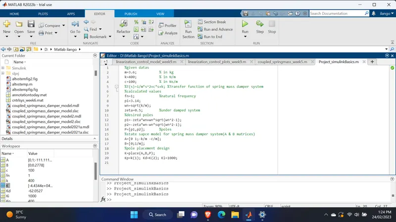
State space model for the spring mass damper system [A & B matrices]

A=[0 1;-k/m -c/m]

B=[0;1/m]

for the desired poles,

p1=-z*wn+z*wn*sqrt(wn^2-1)

p1=-z*wn-z*wn*sqrt(wn^2-1)

P=[p1,p2]

pole placement

K=place(A,B,P)

Matlab Script:

%given datas

m=3.6; % in kg

k=400; % in N/m

c=100; % in Ns/m

%T(s)=1/m*s^2+c*s+k; %Transfer function of spring mass damper system

%calculated values

fn=1; %natural frequency

pi=3.14;

wn=sqrt(k/m);

zeta=0.5; %under damped system

%desired poles

p1=-zeta*wn+wn*sqrt(wn^2-1);

p2=-zeta*wn-wn*sqrt(wn^2-1);

P=[p1,p2]; %poles

%state sapce model for spring mass damper system(A & B matrices)

A=[0 1;-k/m -c/m];

B=[0;1/m];

%pole placement design

K=place(A,B,P);

Kp=k(1); Kd=K(2); Ki=1000;

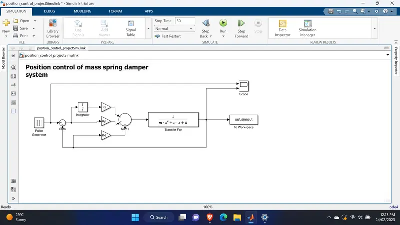
Blocks used:

sum,integrator,transfer function,scope,pulse generator,gain,to workspace.

Pulse generator block:

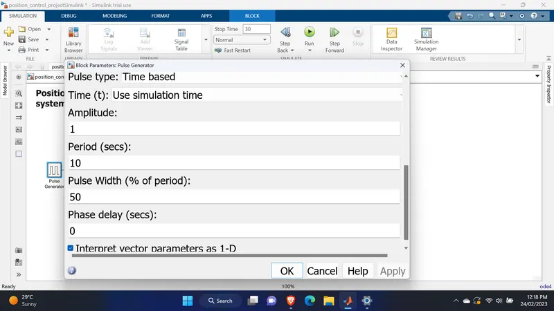
in the given data(diagram), the period(secs) time was there to pick. so took 10 secs from there.

so we can conclude the pulse width 50% of the time(5 secs).

so mentioned the pulse width & the period time.

Transfer function block:

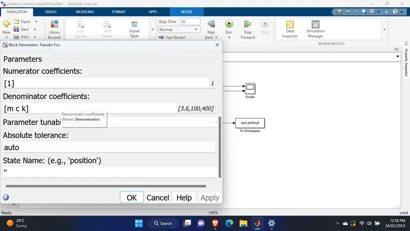
in the transfer function block, mentioned the co efficient values of the term(ms2+cs+k).

the values of m,c & k were given in the question.

Simulation Model:

Here we need to build a simulink model by using transfer function of the spring mass damper system.

we knew that, we will get the transfer function from the differential equation representing the spring mass damper system & its laplace transform.

by pole placement method, using the place command we will get the gain values Kp and Kd.

we need to give the different values for the gain Ki to obtain the better performance.

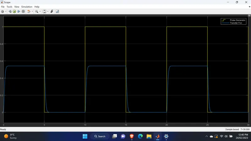
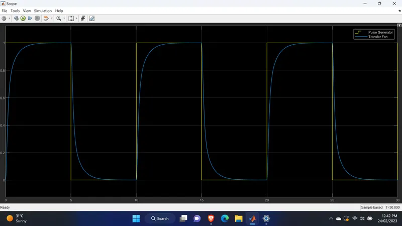
in order to get the better performance took the Ki values as follows, Ki=0, Ki=500, Ki=1000, Ki=2000.,etc

in the integral block took 0 as the initial condition.

simulation was run for 30 seconds.

used the reference value for the pulse generator as per the given data.

used scope block to verify the output.

Practice values 1:

for the gain values

Kp=k(1); Kd=K(2); Ki=0;

Practice values 2:

for the gain values

Kp=k(1); Kd=K(2); Ki=1000;

Practice values 3:

for the gain values

Kp=k(1); Kd=K(2); Ki=2000;

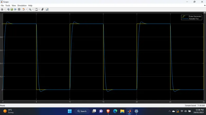
now we can see that the reference signal is closely following the output transfer function signal. over shoot is less than 5%.

increasing the Ki gain value, will give the better performance.

Simulink file was converted to previous version R2021a & uploaded.