Project - Position control of mass spring damper system
- A transfer function is a ratio of output of a system to in input to that system in frequency domain. A practical system consist of many outputs and inputs, dependent and independent. In order to decide this ratio the system output and input quantitiies have to be finalized.
- For a mass spring damper system, the output is preferred as the displacent of the mass in many engineering application (chassi's reference position in case of suspension system of a vehicle) and the input is considered as the force applied to the system (force enccountered due to bumps in road).
- Applying physics laws governing the different theories involved in the system like the Hooke's law to account for the force applied by spring and the Newton's laws of motion to account for the force due to the acceleration of mass and the reaction force to velocity by damper.
- The equations for each force is obtained:
- Force due to Spring, governed by Hooke's Law is given by,
F_spring = k*x(t)
- Force due to the acceleration of mass, governed by Newton's second law of motion is given by,
F_mass = m*D^2[x(t)]
- Force due to the reaction force to velocity by damper, governed by Newton's third law of motion is given by,
F_damper = c*D[x(t)]
here, the quantities are differentiated with respect to time, t.
- Since the total force is equal to the sum of these three forces for a modeled spring-mass-damper system, the forcing function being f(t), the equation represents the force equilibrium condition for the system:
f(t) = F_spring + F_mass + F_damper
f(t) = k*x(t) + m*D^2[x(t)] + c*D[x(t)]
Taking the Laplace equivalent of these equations, we get
F(s) = k*X(s) + m*s^2*X(s) + c*s*X(s)
taking X(s) common,
F(s) = X(s)*(k + m*s^2 + c*s)
X(s)/F(s) = 1/(k + m*s^2 + c*s)
X(s)/F(s) = (1/m)/(s^2 + s* c/m+ k/m)
Thus, we get the transfer function for the mass-spring-damper system in the form of a generic second order system equation.
X(s)/F(s) = (K)/(s^2 +2*zeta*wn+wn^2)
Where,
zeta and wn being damping factor and natural frequency of oscillation,
2*zeta*wn=c/m;
wn=sqrt(k/m);
K=1/m
Visualisation of the current system through online tools:
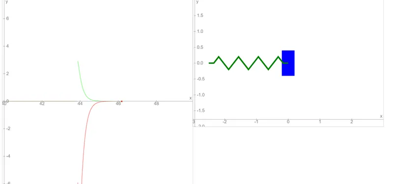
The below link provides the modelled simulation for the current system without the controller. As it can be know by the transfer function, the system is stable. This can be verified by:
The below figure elaborates the behavior of the system for an initial displacement of 3 units.
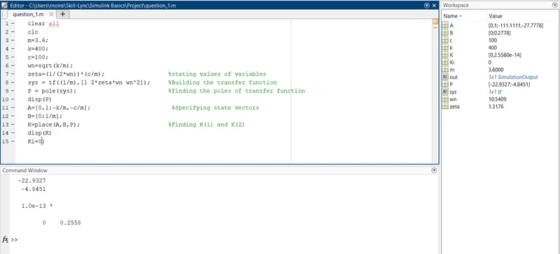
clear all
clc
m=3.6;
k=400;
c=100;
wn=sqrt(k/m);
zeta=(1/(2*wn))*(c/m);                  %stating values of variables
sys = tf((1/m),[1 2*zeta*wn wn^2]);     %Building the transfer function
P = pole(sys);                          %finding the poles of transfer function
disp(P)
A=[0,1;-k/m,-c/m];                       %Specifying state vectors
B=[0;1/m];
K=place(A,B,P);                         %Finding K(1) and K(2)
disp(K)
Ki=0;
negative real values of the poles suggest that the system is highly stable when no forcing function is applied.
In order to perform position control of this system, position being dictated by a rectangular waveform with 50% duty cycle and time period of 10 seconds with unity amplitude, The Kp, Ki and Kd are determined and the error has to be fed to the controller to correct the position of the mass.
A simulink model is built as shown in the screenshot attached below.
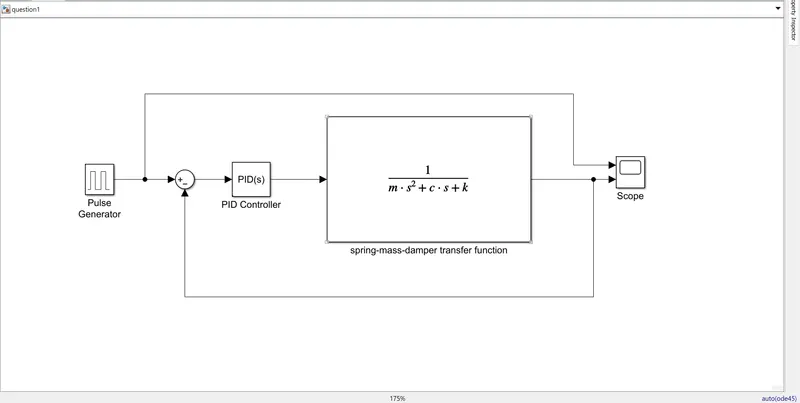
Matlab PID controller block has a built-in tool for the purpose of tuning the Kp, Ki and Kd values.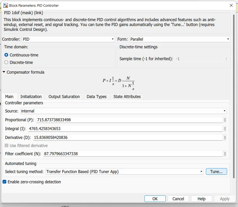
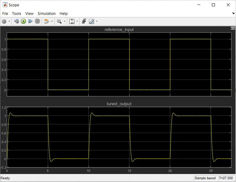
The response of the system is shown.