Project - Mini Project

MobileNetArchitecture:

- MobileNet Architecture is a type Convoluted Neural Network (CNN), which was designed to be efficient, in-order to run on Mobile devices/devices with contrained resources.

- MobileNet Architecture consists of Depth-wise separable Convolution layers (activation of ReLU) stacked with Pooling and Batch Normalisation layers.

What is a CNN?

- A CNN is designed to break down an Input step by step.

- Each subsequent layer breaks down the images, to Narrow down on the features (trainable parameters.) and it analyses each piece individually.

- It learns to recognize complex patterns, and put the pieces back together to make sense of the Input.

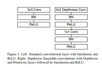
Use of Depth-Wise Convolution Layers:

- Convolution Is performed on a per-channel basis. This improves the feature extraction as each channel's contribution to a feature is learnt whereas in a normal convolution layer, all three channels are consideredon a per-filter basis.

- Pointwise 1x1 convolution is then performed to combine the results of separate where the contribution of each

Use of MaxPooling Layers:

- Pooling layers are used to reduce the size of the Input. This is particularly useful in localizing towards the strong features/patterns within the Input.

(in tensorflow: tf.keras.layers.MaxPoolxD(pool_size)

- This is used to thin down the Neural Network rather than reduce the number of layers.

Use of BatchNormalization layers:

- Batch Normalization layers have two trainable parameters, gamma(scale) and Beta(shift).

- Variance is found out to find the shift of weights, and bought closer to zero. (attempt to reduce variance)

- Scale is calculated in order to optimize the inputs for the next layer. This is to bring them to a format that is more optimized for computation.

Activation Function : ReLU

Relu reduces the input in such a way there are no negative values, so values vary between 0 and max.

- By using a combination of the above layers, MobileNetArchitecture is an approach to efficient onboard computations for embedded operations.

The Need For Data Pre-Processing:

• Each layer in a deep learning model expects a certain input shape for a tensor in order for it to be processed effectively. This is commonly specified at the architectural stage of the model itself. Therefore, models need to have inputs in a certain format.
• Since the mobile net architecture has been trained on ImageNet(process of computing weights that contribute to the end classes.), It can adapt very quickly to non-augmented(non pre-processed) data. which might lead to overfitting and bad generalization.
• Normalising the values between 0 and 1 at the input stage itself, brings improvements to computational efficiency.

Steps taken to pre-process the data:

- Changing th einput shape of the images to (224, 224)

- Rescaling/Normalizing the values between 0 and 1.

- Increasing RandomNess in the data using preprocessing layers from tf.keras.layers:

1. Rescaling (as mentioned above)
2. RandomFlip (flipping the image)
3. RandomZoom(zooming into an image by some factor)
4. RandomHeight(shift height by some factor)
5. RandomWidth(shift width by some factor)
6. RandomRotation(rotate the image by some factor)

Training Process:

Data Loading And Data Augmentation process:

- Load the data into memory using tensorflow.keras.utils.image_dataset_from_directory. Automatically infers the labels/classes from the directory structure.

- Create a Sequential model with keras preprocessing layers.

- Build the model

1. Create the inputs.
2. Augment the Inputs
3. Pass the augmented Inputs to MobilNet
4. Create a Feature Vector using GlobalAvgPool. This layer converts the 2-D spatial information to one dimension feature vector,
5. Interpret Output with Dense layer with single neuron, for binary classification.

The Model is run in inference mode:

- Model is run for 5 epochs (5 times)

- Inference mode means that the layers in the model we have chosen for transfer learning, will be frozen.

- this implies, The weights for all the layers within the model cannot be trained. We will only use the pre-trained weights

- This process is known as Feature extraction.

- The model is specified to not be a top layer (Last most layer, since it needs to access the data early to work and extract the features).

- In this training cycle, Our Pooling layer and Dense layer will be getting trained on the feature vector got from the MobileNEt Model.

Loss Function and Optimizer:

- Since we are working with a Binary Image classification problem, we will be using BinaryCrossEntropy.

- Since MobileNets have good performance with optimizers like RMSprop (RootMeanSquare propogation). Adam can be used as well.

#imports
import tensorflow as tf
from tensorflow import keras
from tensorflow.keras import layers
from tensorflow.keras.optimizers import Adam
from tensorflow.keras.losses import BinaryCrossentropy
import os
import matplotlib.pyplot as plt
import numpy as np

# Fetch the data
current_dir = os.getcwd()
training_dir_name = "cat_dog_data/training_set"
testing_dir_name = "cat_dog_data/test_set"
class_subdirs = ['cats', 'dogs']

training_dir = os.path.join(current_dir, training_dir_name)
testing_dir = os.path.join(current_dir, testing_dir_name)

tf_seed_val = 42

train_data, validation_data = keras.preprocessing.image_dataset_from_directory(training_dir,\
                                                              labels='inferred',\
                                                              color_mode='rgb',\
                                                              image_size=(224 ,224),\
                                                              label_mode="binary",\
                                                              shuffle=True,\
                                                              validation_split=0.5,
                                                              subset="both",
                                                              seed=tf_seed_val)

# Visualise the data
def plot_random_batch_images(data, is_normalised=False):
    """
    Function takes in a random batch and and displays specified number of images.
    data: DataSet/BatchDataSet
    is_normalised: Whether data is normalised. If data is not normalised, works between 0-255 in integer range
        if data is normalised, works with float values
    """
    plt.figure(figsize=(12, 8))
    rand_number = random.randint(0, len(data))
    if is_normalised:
        for images, labels in data.take(rand_number):
            for i in range(9):
                ax = plt.subplot(3, 3, i+1)
                plt.imshow(images[i].numpy())
                plt.title(int(labels[i]))
                plt.axis('off')
    else:
        for images, labels in data.take(rand_number):
            for i in range(9):
                ax = plt.subplot(3, 3, i+1)
                plt.imshow(images[i].numpy().astype('uint8'))
                plt.title(int(labels[i]))
                plt.axis('off')

plot_random_batch_images(train_data, False)

# Create epochs
INIT_EPOCHS = 5

#cehckpoint to save the weights of the model
checkpoint_path="tmp/base_model_v1_checkpoint"

# Create checkpoint callback
save_checkpoint_callback = tf.keras.callbacks.ModelCheckpoint(
    checkpoint_path,
    save_weights_only=True,
    save_freq = "epoch"
)

# Create a Data augmentaion layer
augment_data = keras.Sequential([
    layers.Rescaling(1./255),
    layers.RandomFlip('horizontal_and_vertical'),
    layers.RandomZoom(0.3),
    layers.RandomRotation(0.3),
    layers.RandomHeight(0.2),
    layers.RandomWidth(0.3)
], name="data_augmentation_layer")

# Set up mobile net for inference mode.

from tensorflow.keras.applications import MobileNetV2

mobile_net_base = MobileNetV2(weights="imagenet", # weights pre-trained on ImageNet are loaded.
                              input_shape=(224, 224, 3),
                             include_top=False) # Do not include the ImageNet classifier at the top.

mobile_net_base.trainable = False # Setting the weights of this model to non-trainable.


# Display summary of mobilenetv2 model
print(mobile_net_base.summary())


# Create the model
inputs = layers.Input(shape=(224, 224, 3), name="Input_layer")
x = augment_data(inputs)
x = mobile_net_base(x, training=False)
x = layers.GlobalAvgPool2D(name="gl_avg_pooling_layer")(x)
outputs = layers.Dense(1, activation="sigmoid", name="output_layer")(x)

cd_classifier = keras.Model(inputs, outputs)

#Compile the model
cd_classifier.compile(
    loss=BinaryCrossentropy(), 
    optimizer=tf.keras.optimizers.RMSprop(learning_rate=0.001),
    metrics=["accuracy"])

# Fit the model
new_checkpoint = "tmp/cd_classifier_checkpoint"
cd_checkpoint = keras.callbacks.ModelCheckpoint(new_checkpoint)

cd_history=cd_classifier.fit(
    train_data,
    epochs=INIT_EPOCHS,
    steps_per_epoch=len(train_data),
    validation_data=validation_data,
    validation_steps=int(0.25*len(validation_data)),
    callbacks=[cd_checkpoint]
)

# Plot the loss curves
def plot_loss_curves(model_history):
    """
    Takes in the History of a model. Plots the loss and accuracy. 
    Note current metric used is accuracy, if any other metric is specified
    during model compilation, this function will break. 
    
    Args:
        model_history: History Object of the model
        
    Returns:
        Plots two graphs consisting of loss curves and accuracy curves of model history
    """
    
#     Get values for loss and accuracy
    loss = model_history.history['loss']
    val_loss = model_history.history['val_loss']
    
    accuracy = model_history.history['accuracy']
    val_accuracy = model_history.history['val_accuracy']
    
    epochs = list(range(len(model_history.history['loss'])))
    print(val_loss)
    
#     Plot the loss curves
    plt.figure()
    plt.plot(epochs, loss, label="training_loss")
    plt.plot(epochs, val_loss, label="validation loss")
    plt.title('Model Loss')
    plt.legend();
    
    plt.figure()
    plt.plot(epochs, accuracy, label="training accuracy")
    plt.plot(epochs, val_accuracy, label="validation accuracy")
    plt.title("Model Accuracy")
    plt.legend();

plot_loss_curves(cd_history)

# Evaluate on complete validation set
cd_classifier.evaluate(validation_data)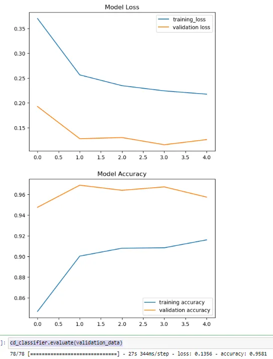

Report:

We can see that in just 5 epochs and limited amount of data, the validation accuracy reaches 96% with the loss being very minimal in inference mode itself.

It also shows that our model is able to generalize its results well and the loss is continuing to decrease.