Project 2

OpenCv new functions used:

1. Gaussian Blur(image, kernel size: list | tuple):
   1. image to blur
   2. kernel size used during convolution
2. convertScaleAbs -> takes in an image, returns the image matrix with values being replaced by absolute values
3. addWeighted(src1, alpha, src2, beta, y):
   1. src1 -> first image
   2. alpha -> weight carried by first image
   3. src2 -> second image
   4. beta -> weight carried by second image
   5. y -> constant
4. Laplacian(src,ddtype, kernel_size):
   1. src: image matrix
   2. type ofdata type in output
   3. kernel size used for convolution

Edge Detection Process Walkthrough:

• First the Image is converted to greyscale as Prewitt Operator works on greyscale images. Good to use same method for laplacian as well
• Image Smoothening/Blurring using Gaussian Filter. Smaller the sigma and kernel size used, reduced smoothening spread, thereby increases the quality of image for edge detection using gradients.
• For Prewitt Operator:
  • Horizontal edge detection kernel (3x3 matrix)is created Gx
    • -1 0 1 row1
    • -1 0 1 row 2
    • -1 0 1 row3
  • Vertical edge detection operator/kernel (3x3 matrix) is created Gy:
    • -1 -1 -1 row1
    • 0 0 0 row 2
    • 1 1 1 row3
  • Filter Image with vertical kernel and horizontal kernel
  • blend the weightage of both these images to get final gradient
• Laplacian Operator is a second order Derivative and measures the rate of change of gradient rather than change in gradient like Prewitt Operator

CODE WALKTHROUGH:

• apply_prewitt_edge_detection:
  • function takes the coloured image matrix
  • converts to Grayscale
  • Apply cv2.GaussianBlur for smoothening image
  • create vertical and horizontal kernel for convolution
  • Convolve the Image with both the kernels
  • finding the absolute values of each of the resultant images using convertScaleAbs, passing the horizontal convolved image and saving it as the horizontal gradient, saving the vertical gradient using the vertically convolved image
  • Now we blend both the images using addWeightage function from cv2. here, both images carry the same weightage (one is not preferred over the other), thereby alpha=beta=0.5. Constant(y) has been ignored in this case
  • the resultant gradient gives us the output for prewitt operator edge detection
• apply_laplacian_filter:
  • Converts image to grey scale
  • takes in image matrix, kernel size and std dev/variance for applying blur operation
  • cv2.Laplacian(grey_image, ddepth=-1, kernel size for laplacian operation)
  • returns the image with edges

import cv2 
import numpy as np 

original_image = cv2.imread('challenge2.png')

"""
 @inputs: 
     original_image: image read by opencv
     kernel_size: size of the kernel to be used in gaussian filter
     sigma: variance/standard deviation to be applied in gaussian blur
 @Ouptut: 
   BW image with edges
"""
def apply_prewitt_edge_detection(original_image, kernel_size, sigma):
    output = cv2.cvtColor(original_image, cv2.COLOR_BGR2GRAY)
    output = cv2.GaussianBlur(output, [kernel_size, kernel_size], sigma)
    vertical_edge_kernel = np.array([[-1, -1, -1], \
                                    [0, 0, 0], \
                                    [1, 1, 1]])
    horizontal_edge_kernel = np.array([[-1, 0, 1], \
                                      [-1, 0, 1], \
                                      [-1, 0, 1]])
    vertical_filtered = cv2.filter2D(output, -1, vertical_edge_kernel)
    horizontal_filtered = cv2.filter2D(output, -1, horizontal_edge_kernel)
    abs_gradient_x = cv2.convertScaleAbs(horizontal_filtered)
    abs_gradient_y = cv2.convertScaleAbs(vertical_filtered)
    gradient = cv2.addWeighted(abs_gradient_x, 0.5, abs_gradient_y, 0.5, 0)
    return gradient

"""
 @inputs: 
     original_image: image read by opencv
     kernel_size: size of the kernel to be used in gaussian filter
     sigma: variance/standard deviation to be applied in gaussian blur
 @Ouptut: BW img with edges
"""
def apply_laplacian_filter(image, kernel_size, sigma):
    output = cv2.cvtColor(original_image, cv2.COLOR_BGR2GRAY)
    output = cv2.GaussianBlur(output, [kernel_size, kernel_size], sigma)
    return cv2.Laplacian(output,-1, kernel_size)

prewitt_edge_image = apply_prewitt_edge_detection(original_image, 3, 3)
cv2.imwrite("prewitt_edge_img.jpg", prewitt_edge_image)
laplacian_edge_image = apply_laplacian_filter(original_image, 3, 3)
cv2.imwrite("laplacian_edge_img.png", laplacian_edge_image)
output_image = np.hstack([prewitt_edge_image, laplacian_edge_image])
cv2.imshow("Edge Detection Comparison", output_image)
cv2.waitKey(0)

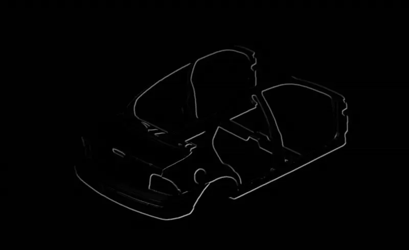
Prewitt Edge Detection output for kernel size 3 and sigma(variance/ std deviation) = 3

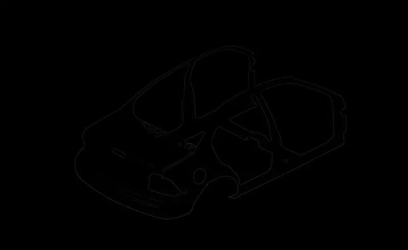
Laplacian with kernel size = 3 and sigma = 3

CONCLUSION:

ON comparing the two images we can see that:

• the image obtained from Laplacian operatin for same kernel size and sigma has more detailed and finer edges.
• Laplacian Image has more details near sections like the A pillar, B pillar and where the edges in general blend in with the background.
• Laplacian operator displays higher sensitivity to gradient changes.
• the above can be verified since the laplacian operator is a second order derivative which is looking at the rate of change of color/gradient where as prewitt is looking for change in color, which explains the thicker edges generated by the prewitt operator

THEREFORE, The edge detection accuracy and better sharpness/detail in edges is higher for Laplacian than prewitt in this case.