Project - Data Handling and Interpolation
Aim:-
In a laboratory experiment, data of voltage and current has been recorded and the same is attached in an excel file ( Click on this link VI.xlsx ). Read the excel file in the Matlab program and perform the interpolation in the range of -17.3:0.1:0.9. Generate the interactive plot for the interpolated data and store them in a text file.
Deliverables:-
Find missing data and save it in text.
Interpolate the data set.
Save your program and attach the same.
Save txt file and upload in attachment.
Solution:-
Interpolation is a mathematical technique to estimate the values of unknown data points that fall in between existing, known data points. You can use interpolation to fill-in missing data, smooth existing data, make predictions, and more. In short, interpolation is a process of determining the unknown values that lie in between the known data points.
In Matlab, interpolation is the procedure of including new points within a defined range or a given set of points. It is used to find the missing data in the data set, smoothen the given data set or predict the outcome of the given data set. Various functions are associated with interpolation techniques. Here, we will mainly discuss one-dimensional interpolation or linear interpolation.
aq=interp1(x, a, xq): The input ‘x’ is a vector that contains every sample point, a has the defined values and xq contains the coordinates. If there are many values, then a can be declared in an array.
aq=interp1(x, a, xq, method): There are many interpolation methods like linear, cubic, spline etc. The default method used is always linear.
There are mainly two types of interpolation methods in Matlab,
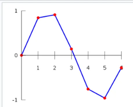
Linear Interpolation Method: This is the default interpolation method used. It helps find the interpolated values at the query point which is based on the values of grid points in each dimension defined. There are certain limitations of this method like 2 points are at least required to use Linear Interpolation.
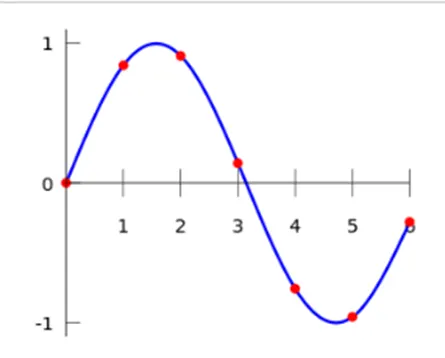
Spline Interpolation Method: This method is used to find the interpolated values using the cubic interpolation of the values. It requires at least four points to find the interpolated values.
Matlab code :-
A=xlsread('voltCurrentData.xlsx'); %reading excel file
v=A(:,1); %separating voltage value
i=A(:,2); %separating current value
xq=[-17.3:0.1:0.9]; %setting interpolation range
yq1=interp1(v,i,xq); %linear interpolated value
yq2=interp1(v,i,xq,'spline'); %spline interpolated value
figure(1)
plot(v,i,'s',xq,yq1,': .'); %ploting linear interpolation
title('Linear interpolation');
xlabel('Voltage [V]');
ylabel('Current [I]');
legend('Actual value','Interpolated value','Location','southeast');
grid on;
figure(2)
plot(v,i,'s',xq,yq2,'m: .');
title('Spline interpolation'); %ploting spline interpolation
xlabel('Voltage [V]');
ylabel('Current [I]');
legend('Actual value','Interpolated value','Location','southeast');
grid on;
val=fopen('voltCurrentData.txt','w'); %opening text file
fprintf(val,' Voltage Current\n');
fprintf(val,'%4.3f %5.3f\n',xq,yq2); %writing voltage & current value
savefig(1,'vilinear.fig'); %saving linear interpolation graph
savefig(2,'vispline.fig'); %saving spline interpolation graph
fclose(val);
Explanation:-
The excel file is read using ‘xlsread ()’ function command
After reading the values of current and voltages are seperated.by using’(:,1)’ and ‘(:,2)’ commands
Then the range of interpolation which has to be done is made as per the question.
The linear interpolation is done using the function ‘Interp1()’ by providing the v, i & interpolation range. Similarly spline interpolation is carried out using the ‘interp1()’ function specifying the method of interpolation as 'spline'.
After performing the interpolation, the plotting is done.
The figure is brought up using the ‘figure ()’ command and plot is done using the ‘plot ()’ command.
The linear interpolation is ploted using the figure(1) command and plot command by providing the actual values of voltage v and current i and the 's' specified the square shape of marker. And the interpolation of the voltage and current also drawn in the same plot by using xq and yq1 with indication of ‘.’
The ‘xlabel ()’ & ‘ylabel ()’ are used for labelling x-axis and y-axis,
Title () command is used for giving the title for the plot
legend () command is used for distinguish the curves, and the it is displayed in the bottom right side by using ‘location’ and then ‘southeast’.
grid is set to on by grid on command.
The spline interpolation curve is ploted with figure(2) and plot command by providing the actual values of voltage v and current i and the 's’ specified the square shape of marker.
Next is the interpolated values of voltage and current which will be shown by small and big dot of magenta color, the m specified indicates the magenta in the plot.
The xlabel() & ylabel() are used for labelling x-axis and y-axis.
title() command is used for giving the title for plot,
legend() l command is used for distinguish the curves, and the it is displayed in the bottom right side by using ‘location’ and then ‘southeast’.
grid is set to on by grid on command.
Now the saving of data and plot created is done, for that a text file called 'voltCurrentData.txt' is opened in write mode using ‘fopen ()’ command.
By using fprintf() command the interpolated values of voltage and current after performing spline interpolation is saved as text file.
Also the plot of linear and spline interpolation were saved in figure format using the savefig() command.
Result:-
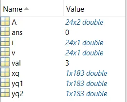
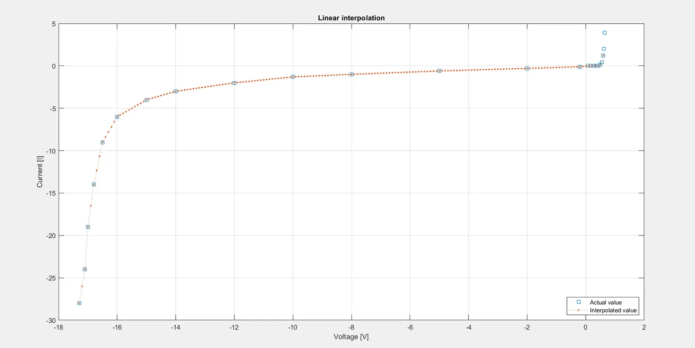
In the plot the square indicates the actual values of voltage and current and dot '.' indicates the interpolation of voltage and current.
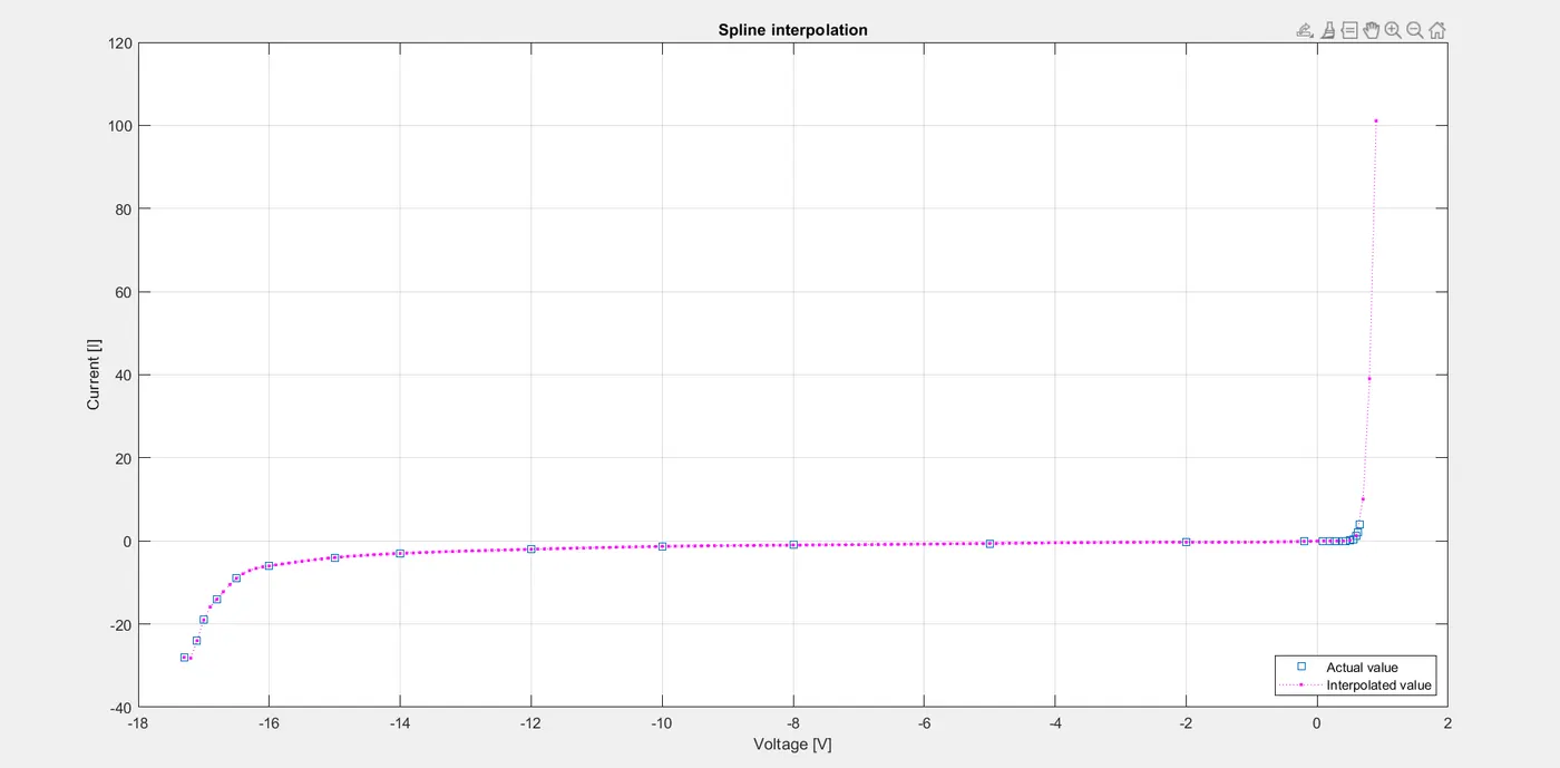
In the plot the square indicates the actual values of voltage and current and dot '.' indicates the spline interpolation of voltage and current.
(The required files are attached below)