Data Handling and Interpolation

Project :

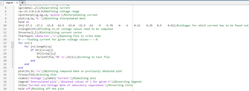
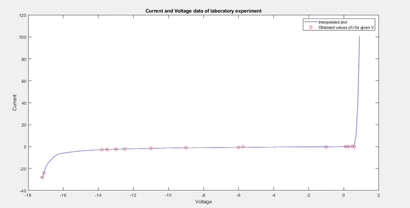
In a laboratory experiment, data of voltage and current has been recorded and the same is attached in an excel file ( VI.xlsx ). Read the excel file in the Matlab program and perform the interpolation in the range of -17.3:0.1:0.9. Generate the interactive plot for the interpolated data. Additionally, compute the current values for given voltages below and store them in a text file.

VV =[-17.2 -17.1 -13.8 -13.5 -13.0 -12.5 -11 -9 -5.76 -6 -1 0.11 0.25 0.5 0.61]’

Key Highlights:

• Graphical solutions are more visual and appealing
• Interpolation of data
• Read excel file
• Write to text file

Interpolation:

Interpolation is a method of fitting data points to represent the value of a function. It has various applications in engineering and science, where it is used to create new data points in a discrete data set of known data points, or it can be used to determine formulas for the (x, y) function that will be passed from a given set of points.

The types of interpolation methods are as follows:

1. linear interpolation
2. Nearest neighbor interpolation or piecewise constant interpolation
3. Polynomial interpolation
4. Spline interpolation
5. Mimetic interpolation
6. Cubic spline interpolation

1. Linear interpolation:

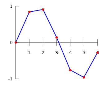
Linear interpolation is a type of interpolation that involves generating new values ​​based on an existing set of values. Linear interpolation is achieved by geometrically drawing a straight line between two adjacent points on a figure or plane. All points on the line except the two initial points can be considered interpolated. Linear interpolation formula

The formula for calculating linear interpolation is as follows:

Linear interpolation (y) = y1+(x−x1) (y2−y1)/(x2−x1)

where

x1 and y1 are the first coordinates
x2 and y2 are the second coordinates
x is the point at which to interpolate
y is an interpolation

2.Nearest neighbor interpolation or piecewise constant interpolation:

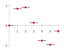
Interpolation is an approximation problem when the value of a function at a given point in some space is given the value of the function at points around this point (adjacent to it). The nearest neighbor algorithm selects the value of the nearest point without even considering the values ​​of neighboring points, resulting in a constant interpolation.

3. Polynomial interpolation:

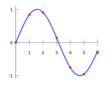
Polynomial interpolation is a method for estimating values ​​between known data points. If there are gaps in the chart data, but the data is on either side of the gap or at several specific points in the gap, the value in the gap can be estimated by interpolation.

4. Spline interpolation:

Spline interpolation, like polynomial interpolation x', takes a polynomial of lower order in each interval and selects segments of the polynomial to fit together smoothly. The resulting function is called a spline.

5. Mimetic interpolation:

Mimetic interpolation is a differential form interpolation method. Unlike other interpolation methods, it estimates the field at a location by considering the values ​​of neighboring points, k{\displaystyle k} simulates the shape of the interpolated calculated field Kk by considering the projection of the field onto neighboring grid elements. Mesh elements can be mesh points as well as cell edges or faces depending on k=0,1,2, 3...{\displaystyle k=0,1,2,\cdots }.

Mimetic interpolation is particularly important in the context of vector and pseudovector fields, as the method preserves line integrals and fluxes, respectively.

6. Cubic spline interpolation:

Cubic spline interpolation is a special case of spline interpolation that is often used to avoid the Runge phenomenon problem. This method provides an interpolation polynomial that is smoother and less error-prone than some other interpolation polynomials, such as Lagrangian polynomials and Newtonian polynomials.

m-script