Project
Aim-Carry out a system-level simulation of an all-terrain vehicle.
Objective-Prepare a technical report explaining the model properties & comments on the results.
Theory-
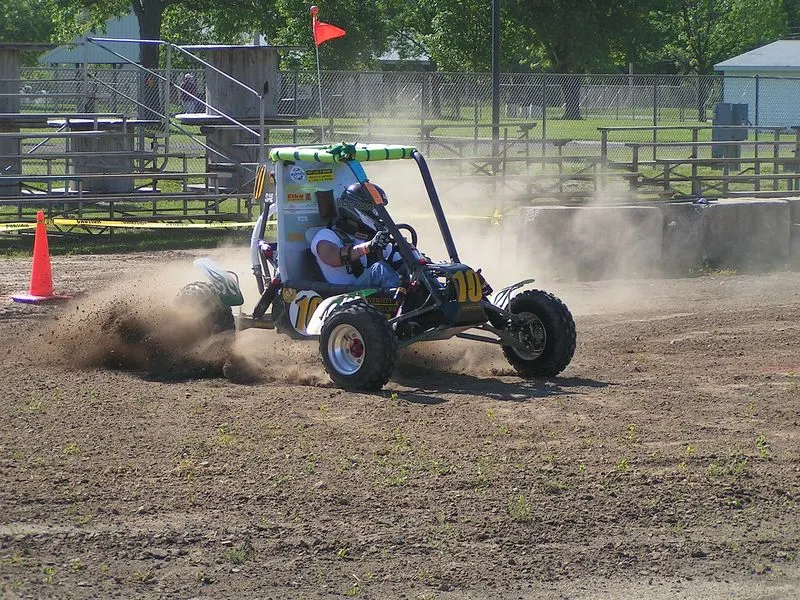
An all-terrain vehicle (ATV), also known as a light utility vehicle (LUV),a quad bike, or simply a quad, as defined by the American National Standards Institute (ANSI); is a vehicle that travels on low-pressure tires, with a seat that is straddled by the operator, along with handlebars for steering control. As the name implies, it is designed to handle a wider variety of terrain than most other vehicles. Although it is a street-legal vehicle in some countries, it is not street-legal within most states, territories and provinces of Australia, the United States or Canada.
By the current ANSI definition, ATVs are intended for use by a single operator, although some companies have developed ATVs intended for use by the operator and one passenger. These ATVs are referred to as tandem ATVs.
The rider sits on and operates these vehicles like a motorcycle, but the extra wheels give more stability at slower speeds. Although most are equipped with three or four wheels, six-wheel models exists and existed historically for specialized applications. Multiple-user analogues with side-by-side seating are called utility terrain vehicles (UTVs) or side-by-sides to distinguish the classes of vehicle. Both classes tend to have similar powertrain parts. Engine sizes of ATVs currently for sale in the United States (as of 2008 products) range from 49 to 1,000 cc (3.0 to 61 cu in).
Continuously variable transmission (CVT) -
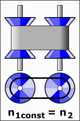
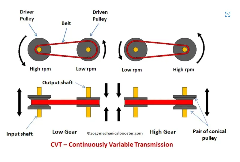
A continuously variable transmission (CVT) is an automatic transmission that can change seamlessly through a continuous range of gear ratios. This contrasts with other transmissions that provide a limited number of gear ratios in fixed steps. The flexibility of a CVT with suitable control may allow the engine to operate at a constant RPM while the vehicle moves at varying speeds.CVTs are used in automobiles, tractors, motor scooters, snowmobiles, bicycles and earthmoving equipment.The most common type of CVT uses two pulleys connected by a belt or chain; however, several other designs have also been used at times.
Working of CVT
The manual and automatic transmission systems have complex working which depends upon gear shifting. There, two gears can achieve gear ratio, but in CVT two pulleys mechanism provides not only a single gear ratio but countless or infinite gear ratio. Both are connected by a push belt, one pulley (Primary) is connected with the engine and another (Secondary) pulley with a drive shaft. Each pulley attached with a moveable sheave which causes expansion and contraction of the pulleys at both ends. As the engine turns the primary pulley and secondary pulley diameter size gets changed due to moving sheaves of both pulleys. If one pulley’s size is decreased, at the same time the second pulley’s size is increased and vice versa. The size variation of pulleys means diameters also varies which creates the continuous gear ratios. In manual gearbox input and output gear teeth decides the ratios, but here variation in diameter decides the ratios.
BAJA ATV Vehical Model
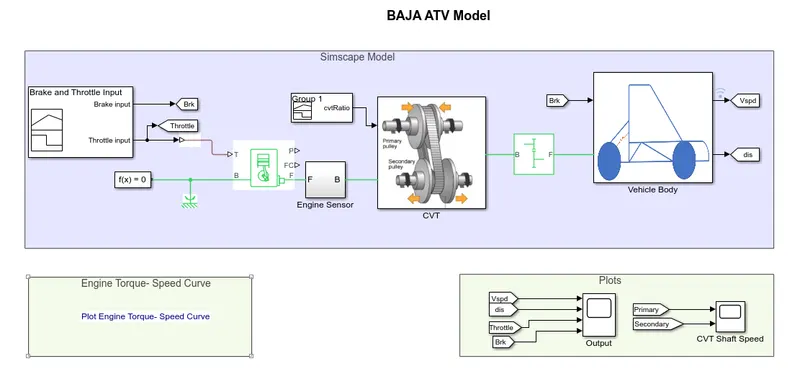
Main Components Of BAJA ATV as FOLLOWS
1)Genetic Engine
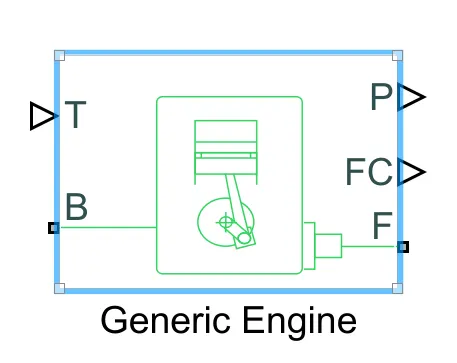
Represents a system-level model of spark-ignition and diesel engines suitable for use at initial stages of modeling when only the basic parameters are available. Optional idle speed and red line controllers are included.
The throttle input signal T lies between zero and one and specifies the torque demanded from the engine as a fraction of the maximum possible torque. If the engine speed falls below the Stall speed, the engine torque is blended to zero. If the engine speed exceeds the Maximum speed, the simulation stops and issues an error message.
Connections F and B are mechanical rotational conserving ports associated with the engine crankshaft and engine block, respectively. Connections P and FC are physical signal output ports through which engine power and fuel consumption rate are reported.
Signal ports
B – Rotational Conserving Port representing the Engine Block
F – Rotational Conserving Port representing the Engine Crankshaft
T - Physical signal input port specifying the normalized engine throttle level
P - Physical signal output port reporting the instantaneous engine power, in W
FC - Physical signal output port reporting the fuel consumption rate, in kg/s
2)Engine Sensors
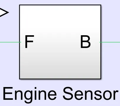
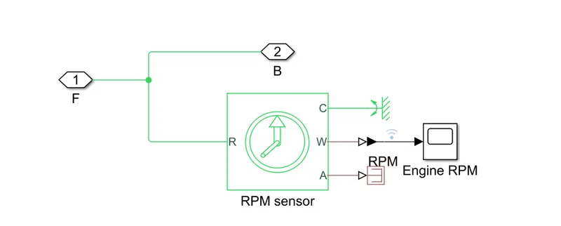
Engine sensor block connected the out port port of generic engine 'F'.Engine sensor block contains the ideal rotation sensor block.This block measures angular velocity or angle in a mechanical rotational network. The sensor is ideal since it does not account for inertia, friction, delays, energy consumption, and so on.
3)Simple Gear
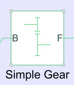
Represents a fixed-ratio gear or gear box. No inertia or compliance is modeled in this block. You can optionally include gear meshing and viscous bearing losses.
Connections B (base) and F (follower) are mechanical rotational conserving ports. Specify the relation between base and follower rotation directions with the Output shaft rotates parameter. Optionally include thermal effects and expose thermal conserving port H by setting Friction model to a temperature-dependent setting.
4)CVT TRANSMISSION Block
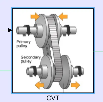
CVT Block is sub system contains many blocks of Variable drive System.The image of CVT transmission pully is added on block by ''MASK''command in simulink.CVT subsystem cointains following blocks.
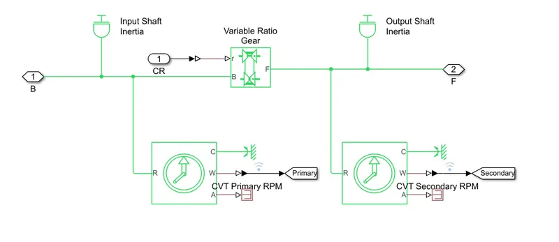
CVT subsystem contains the two inertia blocks for input and out put shaft.To measure Input output speed there is two rotational motion sensors.
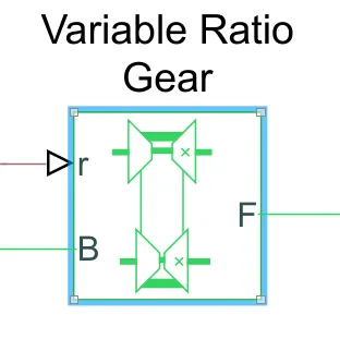
Represents a variable ratio gearbox such as implemented by mechanical belt CVT, electric, or hydraulic transmissions. The physical signal input r defines the ratio of input to output angular shaft velocities.
Connections B (base) and F (follower) are mechanical rotational conserving ports. Specify the relation between base and follower rotation directions with the Output shaft rotates parameter.
B – Base Pulley or Drive Pulley
F – Follower Pulley or Driven Pulley
r – Variable Transmission Ratio (Input)
5) Vehical Body subsystem
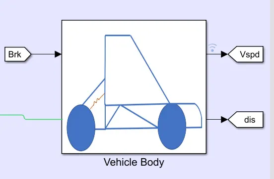
The subsystem vehical body contain many blocks.It contains wheels, bracks,body.
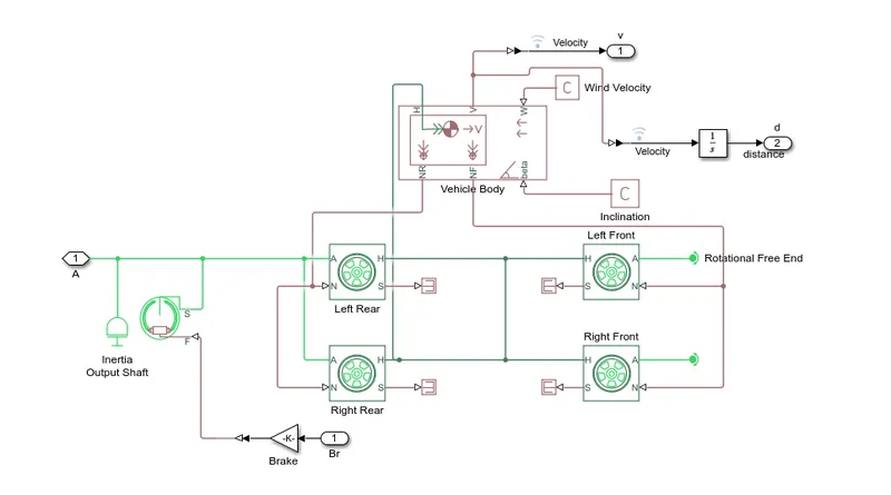
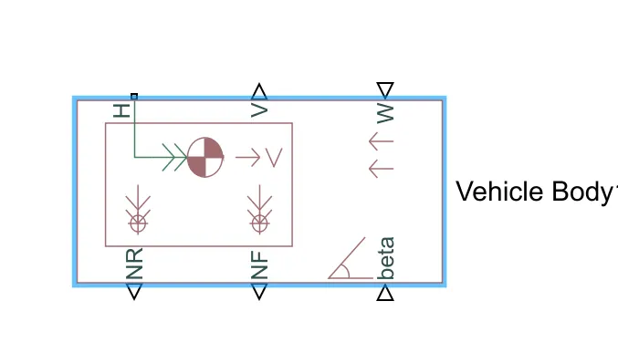
Two-axle vehicle with longitudinal dynamics and motion and adjustable mass, geometry, and drag properties. The
vehicle can have the same or a different number of wheels on each axle. For example, two wheels on the front axle and one wheel on the rear axle. The vehicle wheels are assumed identical in size. The vehicle can also have a centre of gravity (CG) that is at or below the plane of travel.
Connection H is the mechanical translational conserving port associated with the horizontal motion of the vehicle body. The resulting traction motion developed by tires should be connected to this port. Connections V, NF, and NR are physical signal output ports for vehicle velocity and front and rear normal wheel forces, respectively. Wheel forces are considered positive if acting downwards. Connections W and beta are physical signal input ports corresponding to headwind speed and road inclination angle, respectively. If variable mass is modeled, the physical signal input ports CG and M are exposed. CG accepts a two- element vector representing the x and y distance offsets from vehicle CG to additional load mass CG. M represents the additional mass. If both variable mass and pitch dynamics are included, the physical signal port J accepts the inertia of the additional mass about its own CG.
NR – Rear Axle Normal Force (N)
NF – Front Axle Normal Force (N)
Beta – Road Incline Angle (rad)
V – Longitudinal Velocity (m/s)
W – Head Wind Speed (m/s)
H – Horizontal Motion
6)Double shoe Brake
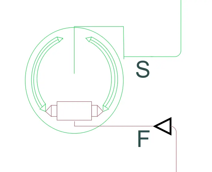
Represents a brake arranged as two pivoted rigid shoes symmetrically installed inside or outside a drum and operated by one actuator. The actuator force causes the shoes to exert a friction torque on a shaft connected to the drum.
Connection S is a conserving rotational terminal associated with the drum shaft. Connection F is a physical signal port representing the force input to the actuator. Positive force creates friction torque that resists shaft rotation. Optionally include thermal effects and expose thermal conserving port H by setting Thermal port to Model.
7)Tire Magic formula
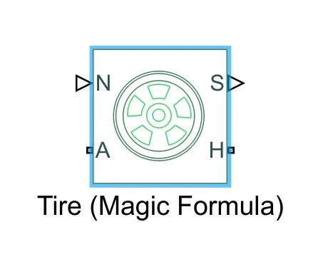
Represents the longitudinal behavior of a highway tire characterized by the tire Magic Formula. The block is built from Tire-Road Interaction (Magic Formula) and Simscape Foundation Library Wheel and Axle blocks. Optionally, the effects of tire inertia, stiffness, and damping can be included.
Connection A is the mechanical rotational conserving port for the wheel axle. Connection H is the mechanical translational conserving port for the wheel hub through which the thrust developed by the tire is applied to the vehicle. Connection N is a physical signal input port that applies the normal force acting on the tire. The force is considered positive if it acts downwards. Connection S is a physical signal output port that reports the tire slip. Optionally expose physical signal port M by setting Parameterize by to Physical signal Magic Formula coefficients. Physical signal port M accepts a four element vector corresponding to the B, C, D, and E Magic Formula coefficients.
N – Normal Force
S – Tire Slip
A – Axle
H – Mechanical translational port associated with the wheel hub that transmits the thrust generated by the tire to the remainder of the vehicle.
General Blocks Used
Signal Builder – To input the Brake, Throttle and CVT Ratio.
Simulink to PS Converter – To convert the Simulink signal to Simscape environment.
Solver Configuration – To specify the solver parameters before starting the simulation.
Mechanical Reference – To make sure all the components are clamped to the ground.
Generic Engine – To run the engine with speed and torque values as input.
PS to Simulink Converter – To convert Simscape signal to Simulink environment.
Scope – To view the graph of the parameters for better understanding.
Display – To view the calculated engine power.
Inertia – To represent the solid inertia.
Rotational Motion Sensor – To sense the rotational motion from the engine and give output as rpm.
Variable Gear Ratio – To vary the speed according to the gear ratios.
PS Terminator - Terminator for unconnected physical signal outputs.
Double Shoe Brake – To apply brake to the vehicle when needed.
PS Constant - Generate constant physical signal.
Tire – For transportation of the vehicle.
Rotational Free End – For mechanical component (Tire).
Vehicle Body – To represent the BAJA ATV model body.
Custom Measure Gauge – To measure the brake and throttle input.
Knob – To increase, decrease and vice-versa of throttle and brake inputs.
Lookup Table – To insert the CVT values from the workspace.
Simple Gear – To reduce the speed of the engine with pre-defined gear ratio.
Step – To increase or decrease an input value for a defined time interval.
TYPES OF MODEL :-
BAJA ATV model without Dashboard
BAJA ATV model with Dashboard
BAJA ATV model - Lookup Table Data Extraction
BAJA ATV model – Mapped Lookup Table without Dashboard
BAJA ATV model – Mapped Lookup Table with Dashboard
FLOW PROCESS :-
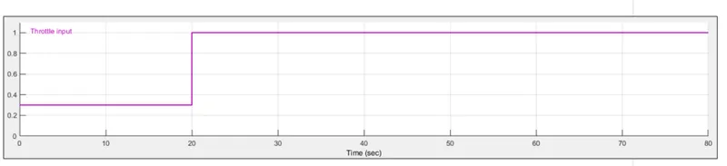
i.The throttle signal is generated by signal builder block and input to generic engine.
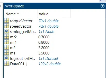
ii.The torque and speed vector are inputted from the MATLAB workspace.
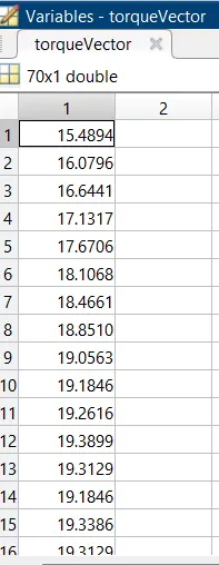
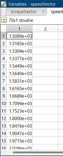
iii.The engine will generate the output rpm which can be taken from the crankshaft output. This speed will be given to the Ideal Rotational Motion Sensor to sense the output rpm.
iv.The same output speed will be given to a simple gear mechanism to reduce the speed where the Gear Ratio is ‘4’.
v.Then the output speed from the gear reducer will be given to the Variable Ratio Transmission block (CVT).
vi.The CVT ratio is provided to the Variable Ratio Transmission (CVT) block through Signal Builder.
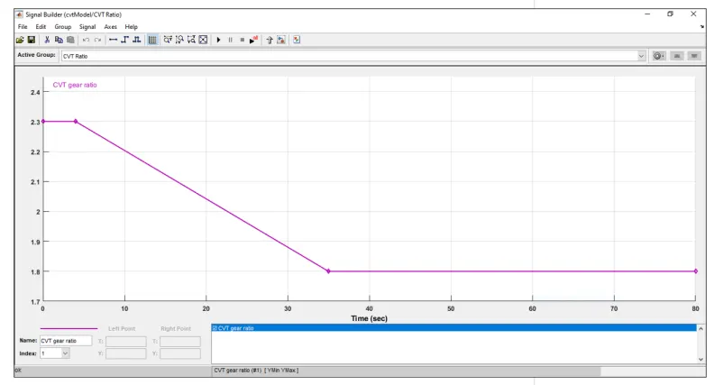
vii.The speed is controlled by the variable CVT ratios and the controlled output speed is inputted to the vehicle axle.
viii.The brake signal is generated by the signal builder and inputted to the vehicle body (Double Shoe Brake) for applying the brake to axle.

ix.The power from the CVT is inputted to the axle and the vehicle accelerates according to the speed.
x.Then the Velocity is taken as output from the vehicle body for further analysis.
SPeed Vs Trottle Plot
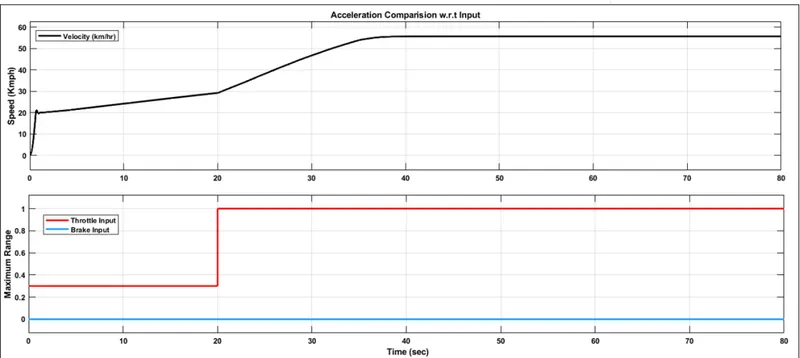
From the graph we can infer that the brake is not applied during the drive cycle and the Throttle is constant (0.3) till 20 sec and being increased from 0.3 to 1 from 20 sec where it remains constant throughout. With increase in throttle the vehicle speed also increases.
ENGINE SPEED vs GEAR REDUCTION SPEED PLOT,
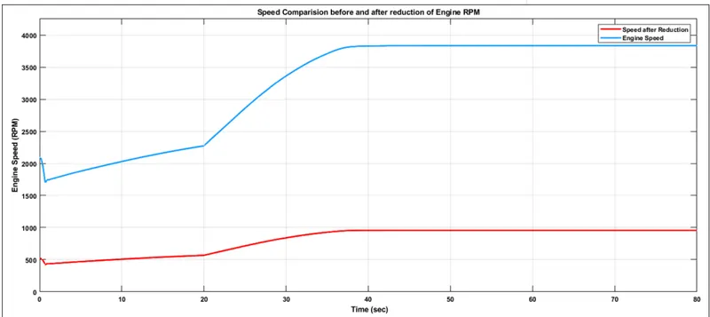
Here we can see that the engine speed is reduced by the Gear Ratio ‘4’. For verification I calculated the maximum RPM,
Maximum RPM (Before Reducing) = 3833 rpm
Gear Ratio = 1:4
CVT SPEED REDUCTION PLOT,
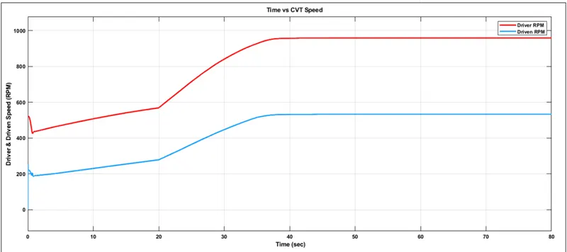
The engine reduced speed is controlled by various CVT Ratios. For verification I had calculated the maximum RPM,
Maximum RPM (Before Reducing) = 958.25 rpm
CVT Ratio = 1:1.8
SPEED vs THROTTLE PLOT,
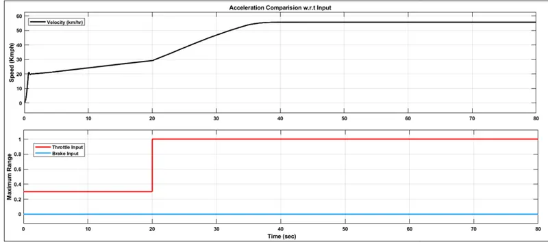
From the graph we can infer that the brake is not applied during the drive cycle and the Throttle is constant (0.3) till 20 sec and being increased from 0.3 to 1 from 20 sec where it remains constant throughout. With increase in throttle the vehicle speed also increases.
ACCELERATION PLOT,
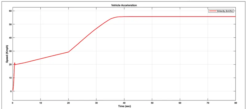
From the above plot we can infer that the vehicle is accelerated from 0-20 Kmph and then gradually increases then it’s accelerated to 55.74 Kmph where it remains constant throughout the cycle.
BAJA MODEL WITH DASHBOARD
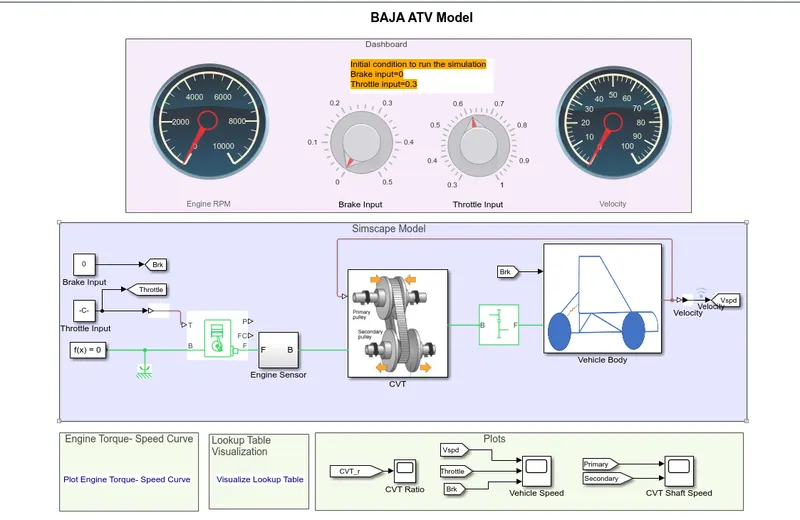
The model workflow process is same as the process of ‘BAJA ATV model without Dashboard’ but the Throttle and Brake
inputs are controlled by the user with the Knob.
ENGINE SPEED PLOT
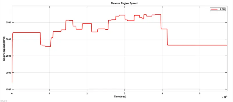
Here the engine speed is generated according to the inputs like throttle, break, torque and speed vectors. The runtime is not defined so that the Throttle and Break are controlled by the user. The step up is throttle and step down are break inputs.
ENGINE SPEED vs GEAR REDUCTION SPEED PLOT,
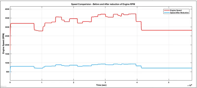
Here we can see that the engine speed is reduced by the Gear Ratio ‘4’. For verification I calculated the constant RPM (42000-50000
sec),
Maximum RPM (Before Reducing) = 2759.3 rpm
Gear Ratio = 1:4
CVT SPEED REDUCTION PLOT
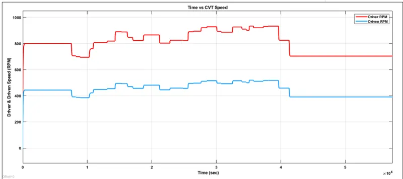
The engine reduced speed is controlled by various CVT Ratios. For verification I had calculated the constant RPM (42000-50000 sec),
Maximum RPM (Before Reducing) = 689.825 rpm
CVT Ratio = 1:1.8
SPEED vs THROTTLE PLOT,
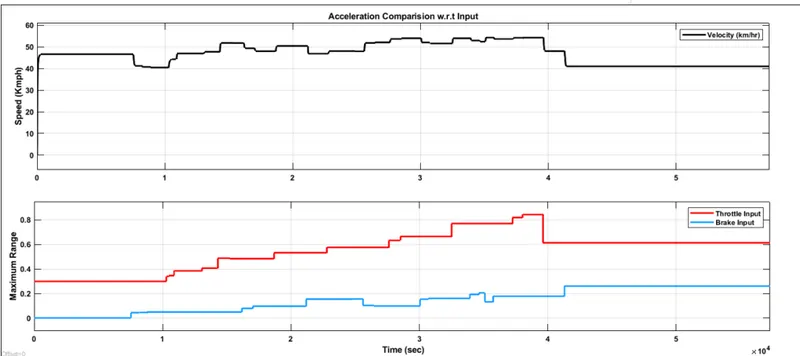
From the graph we can infer that the vehicle is accelerating while throttle is applied (Step Up) and decelerated while break is applied (Step Down).
ACCELERATION PLOT,
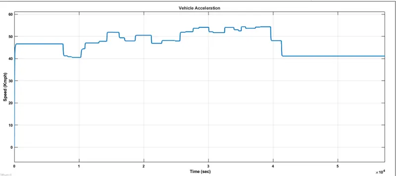
rom the graph we can infer that the vehicle is accelerated to 46 Kmph initially and then the state changes when the user controls the throttle and brake knobs. The step-up and step-down are acceleration and deceleration respectively. The linear one is the constant speed so no changes in throttle or braking.
SIMULINK MODEL
i. https://in.mathworks.com/matlabcentral/fileexchange/70576-baja-all-terrain-vehicle-atv-model
REFERENCES
https://in.mathworks.com/videos/modeling-a-vehicle-with-continuously-variable-transmission-1554467867519.html?
fbclid=IwAR2NqnIVVLAhrP3TNWoV1WkkmZd0UofkkTIu5fGI2XPwd5T7w7x4QF6oeiU
https://www.pathwayz.org/Tree/Plain/FORCES+-+NAMES+AND+DIAGRAMS
https://in.mathworks.com/help/physmod/sdl/ref/tiremagicformula.html
https://in.mathworks.com/help/physmod/sdl/ref/doubleshoebrake.html#:~:text=Double%2Dshoe%20brakes%20provide
https://bajasaeindia.org/downloads.html