Project on system level simulation of an ATV

Project on ATV Simulation

Aim: To carry out a system level simulation of a Simulink based model of an All-Terrain Vehicle

The model: https://www.mathworks.com/matlabcentral/fileexchange/70576-baja-all-terrain-vehicle-atv-mode

Description

In the given project, we have been tasked to simulate and analyse a Simulink based model of an All-Terrain Vehicle(ATV). The model is built for an ATV that is compatible for participation in the intercollegiate competition of SAE-BAJA. Let’s know both these terms at first:

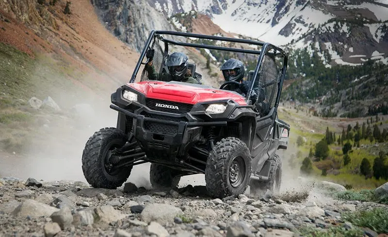
All-Terrain Vehicle: An all-terrain vehicle (ATV), also known as a light utility vehicle (LUV), a quad bike, or simply a quad, as defined by the American National Standards Institute (ANSI); is a vehicle that travels on low-pressure tires, with a seat that is straddled by the operator, along with handlebars for steering control. As the name implies, it is designed to handle a wider variety of terrain than most other vehicles.By the current ANSI definition, ATVs are intended for use by a single operator, although some companies have developed ATVs intended for use by the operator and one passenger. These ATVs are referred to as tandem ATVs. The rider sits on and operates these vehicles like a motorcycle, but the extra wheels give more stability at slower speeds. Although most are equipped with three or four wheels, six-wheel models exists and existed historically for specialized applications.

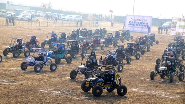
SAE BAJA: Baja SAE is an Collegiate Design Series competition run by the Society of Automotive Engineers International (SAE International). Teams of students from universities all over the world design and build small off-road cars. The cars all have engines of the same specifications. The goal in Baja SAE racing is to design, build and race off-road vehicles that can withstand the harshest elements of rough terrain. The vehicles used in Baja SAE racing are often similar in appearance to dune buggies. Before 2007, the events were called "Mini Baja." All cars must adhere to SAE International's rules, and pass SAE's technical inspection and judging; a car may not race until all safety inspections are passed.

Let’s now know about the model/s under consideration here. There are various models built in here with similar construction of the vehicle body but with different input conditions for all. The models under study are:

A) ATV model with signal builder inputs for brake, throttle and CVT.

B) ATV model with a dashboard facilitating dynamic inputs via knobs.

C) ATV model with output of the axle mapped as an input to the CVT block.

D) ATV model with output of the axle mapped as an input to the CVT block with a dashboard facilitating knobs for dynamic input.

The vehicle body of all these models though is same. Let’s have a look at the model:

Blocks/components used:

1) Signal builder

2) Solver configuration

3) Mechanical Rotational Reference

4) Generic Engine

5) Ideal Rotational Motion Sensor

6) Inertia

7) Variable Ratio Transmission

8) PS Terminator

9) Inport

10) Simulink to PS converter

11) PS to Simulink Converter

12) Tire (Magic Formula)

13) Double Shoe Brake

14) Gain

15) PS Constant

16) Integrator

17) Outport

18) Goto

19) From

20) Scope

21) Knob

22) Circular Gauge

23) PS Lookup Table

24) Step

25) Simple gear

The models

A) ATV model with inputs from signal builder for brake, throttle and CVT

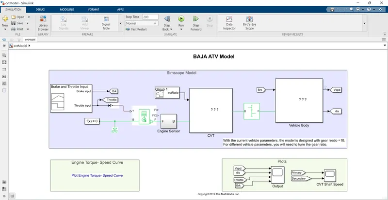
The above displayed model is the most basic of all the models. The components comprising it are:

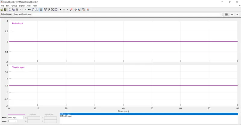
1) Signal Builder - The Signal Builder block allows you to create interchangeable groups of piecewise linear signal sources and use them in a model. You can quickly switch the signal groups into and out of a model to facilitate testing. In the Signal Builder window, create signals and define the output waveforms. To open the window, double-click the block. This block is configured as:

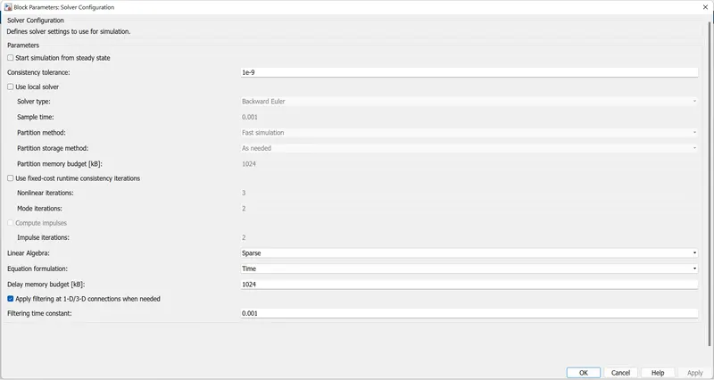
2) Solver Configuration - Defines solver settings to use for simulation. This block is configured as:

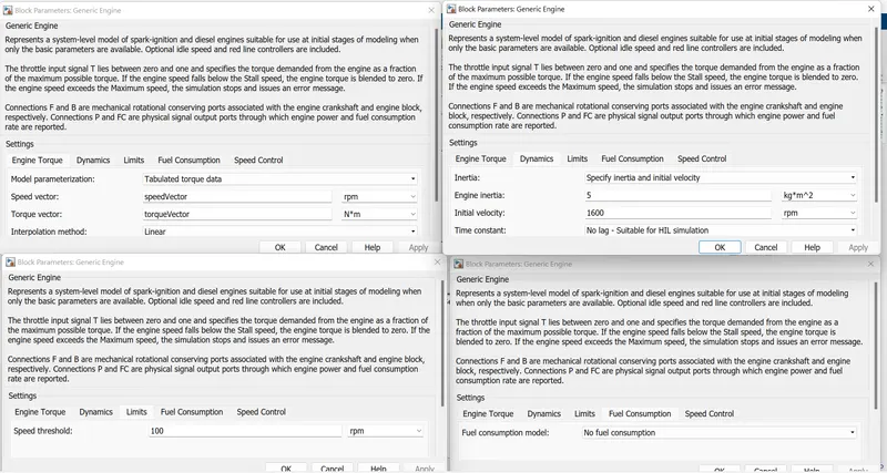
3) Generic Engine - Represents a system-level model of spark-ignition and diesel engines suitable for use at initial stages of modelling when only the basic parameters are available. Optional idle speed and red line controllers are included.The throttle input signal T lies between zero and one and specifies the torque demanded from the engine as a fraction of the maximum possible torque. If the engine speed falls below the Stall speed, the engine torque is blended to zero. If the engine speed exceeds the Maximum speed, the simulation stops and issues an error message.Connections F and B are mechanical rotational conserving ports associated with the engine crankshaft and engine block, respectively. Connections P and FC are physical signal output ports through which engine power and fuel consumption rate are reported. This block is configured as:

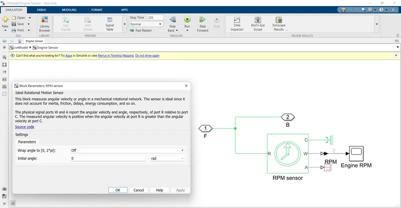
4) Engine Sensor – This block is the subsystem of an ideal rotational motion sensor which measures angular velocity or angle in a mechanical rotational network. The sensor is ideal since it does not account for inertia, friction, delays, energy consumption, and so on. The physical signal ports W and A report the angular velocity and angle, respectively, of port R relative to port C. The measured angular velocity is positive when the angular velocity at port R is greater than the angular velocity at port C. This block is configured as:

5) CVT – This is a subsystem representing the CVT of an automobile. It has the following blocks:

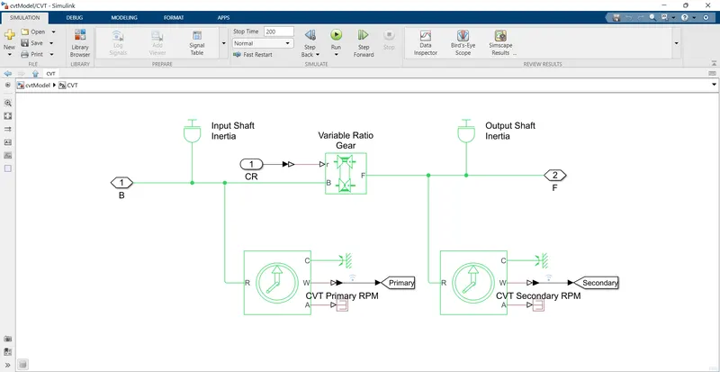
Inertia - The block represents an ideal mechanical rotational inertia. The block has one or two mechanical rotational conserving ports. The difference is purely graphical, as the ports are rigidly linked. The block positive direction is from its port to the reference point. This means that the inertia torque is positive if the inertia is accelerated in the positive direction. Two such blocks are used, one for the input shaft while the other for the output shaft. This block is configured as:

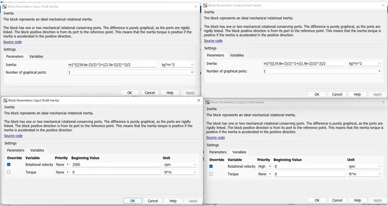
Ideal Rotational Motion Sensor – Two of these blcoks are used, one representing the primary pulley whereas the other representing the secondary pulley. This block is configured as shown above.

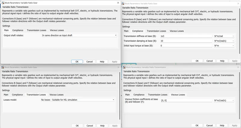
Variable Ratio Transmission - Represents a variable ratio gearbox such as implemented by mechanical belt CVT, electric, or hydraulic transmissions. The physical signal input r defines the ratio of input to output angular shaft velocities.Connections B (base) and F (follower) are mechanical rotational conserving ports. This block is configured as:

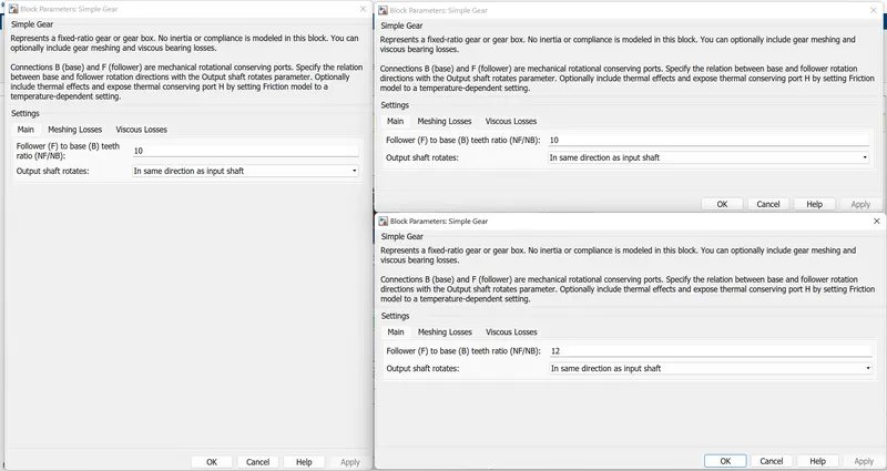
6) Simple Gear - Represents a fixed-ratio gear or gearbox. No inertia or compliance is modelled in this block. You can optionally include gear meshing and viscous bearing losses. Connections B (base) and F (follower) are mechanical rotational conserving ports. This block is configured as:

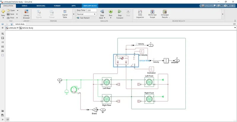
7) Vehicle body – Again this is a subsystem comprising of:

Inertia – The same block as discussed above. This block is configured as:

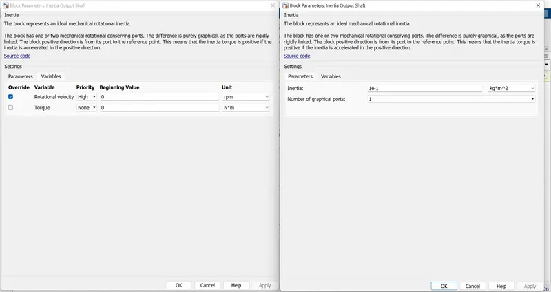
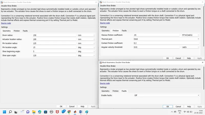
Double shoe brake - Represents a brake arranged as two pivoted rigid shoes symmetrically installed inside or outside a drum and operated by one actuator. The actuator force causes the shoes to exert a friction torque on a shaft connected to the drum.Connection S is a conserving rotational terminal associated with the drum shaft. Connection F is a physical signal port representing the force input to the actuator. Positive force creates friction torque that resists shaft rotation. Optionally include thermal effects and expose thermal conserving port H by setting Thermal port to Model. This block is configured as:

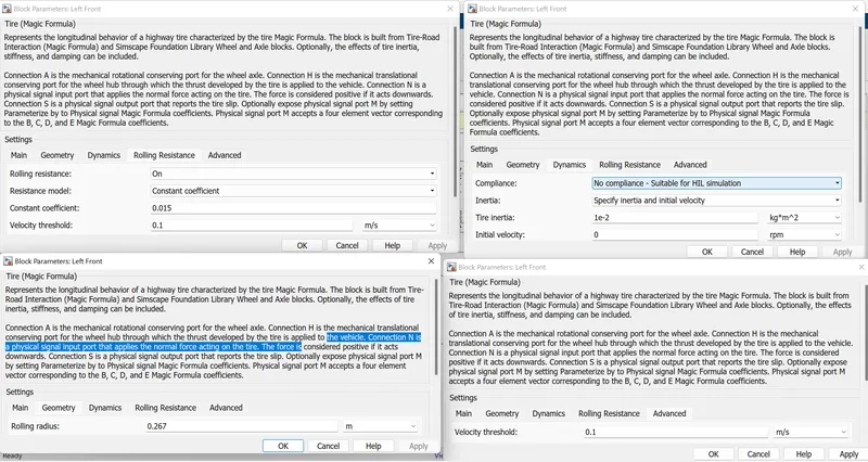
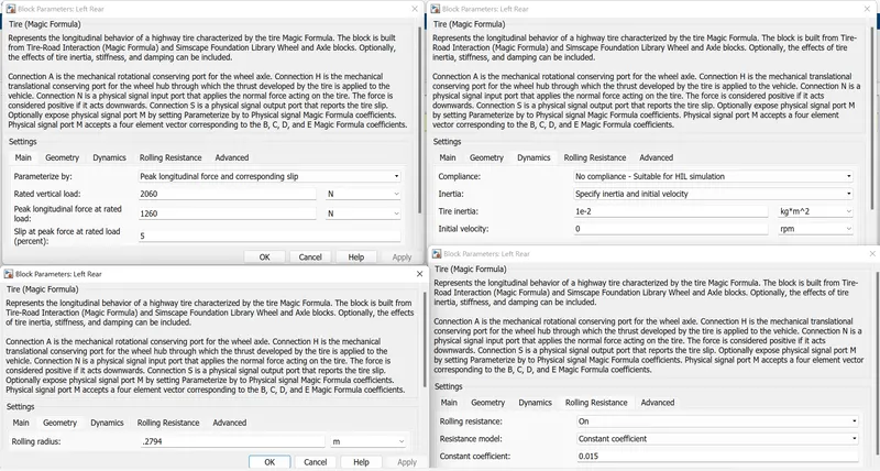
Tire - Represents the longitudinal behaviour of a highway tire characterized by the tire Magic Formula. The block is built from Tire-Road Interaction (Magic Formula) and Simscape Foundation Library Wheel and Axle blocks. Optionally, the effects of tire inertia, stiffness, and damping can be included.Connection A is the mechanical rotational conserving port for the wheel axle. Connection H is the mechanical translational conserving port for the wheel hub through which the thrust developed by the tire is applied to the vehicle. Connection N is a physical signal input port that applies the normal force acting on the tire. The force is considered positive if it acts downwards. Connection S is a physical signal output port that reports the tire slip. Optionally expose physical signal port M by setting Parameterize by to Physical signal Magic Formula coefficients. Physical signal port M accepts a four element vector corresponding to the B, C, D, and E Magic Formula coefficients.

Four of these blocks are used, representing the four wheels of the ATV. The H ports of the left front tire and left rear tire are connected with each other and similarly for the right tires as well. Both these connections are then connected to the H port of the Vehicle body block. ‘A’ ports of the rear tires are connected to the input shaft while those of the front tires are connected to the rotational free end. The N ports receive their inputs from the Vehicle body block. The S ports meanwhile are connected to the PS terminator blocks. These blocks are configured as:

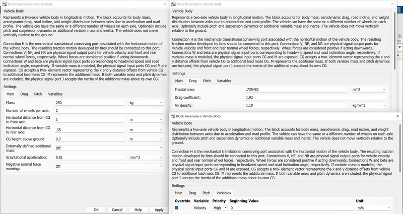
Vehicle Body - Represents a two-axle vehicle body in longitudinal motion. The block accounts for body mass, aerodynamic drag, road incline, and weight distribution between axles due to acceleration and road profile. The vehicle can have the same or a different number of wheels on each axle. Optionally include pitch and suspension dynamics or additional variable mass and inertia. The vehicle does not move vertically relative to the ground.Connection H is the mechanical translational conserving port associated with the horizontal motion of the vehicle body. The resulting traction motion developed by tires should be connected to this port. Connections V, NF, and NR are physical signal output ports for vehicle velocity and front and rear normal wheel forces, respectively. Wheel forces are considered positive if acting downwards. Connections W and beta are physical signal input ports corresponding to headwind speed and road inclination angle, respectively. If variable mass is modelled, the physical signal input ports CG and M are exposed. CG accepts a two- element vector representing the x and y distance offsets from vehicle CG to additional load mass CG. M represents the additional mass. If both variable mass and pitch dynamics are included, the physical signal port J accepts the inertia of the additional mass about its own CG.

The N and H ports are connected as discussed in the above block. The w port is for the wind which in case of high wind velocities can be assigned the appropriate values, but in our case we take it to be zero. Similarly, the b port can be provided with hill climb inclination but for our case it is taken to be zero. The velocity as an output is taken from the v port and on integrating this value we can obtain the displacement as well. This block is configured as:

Output Results:

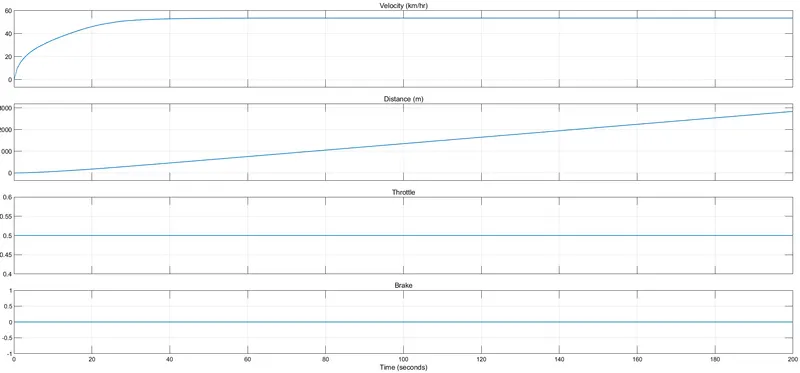
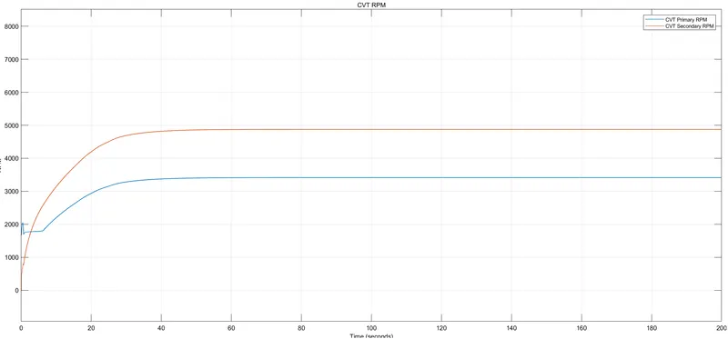
As can be seen, for a constant throttle of 0.5 the vehicle first accelerates and attains a maximum speed of 53.532 kmph and then maintains this constant speed thereafter. The brake during this cycle is kept at 0 (no braking). The total distance traveled during this time is 2838 m. The CVT secondary rpm meanwhile follows trail, increases at first attains a maximum of 4880 and stays constant thereafter.

B) ATV model with a dashboard facilitating dynamic inputs via knobs.

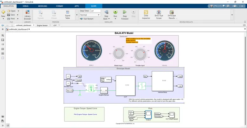
The only difference between the model in 'A' and this model is that the throttle and brake inputs here are provided as dynamic inputs via knobs that can be tuned while the simulation is running. In addition, the change in RPM and velocity can be viewed on the circular guages of the dashboard.

Output Results

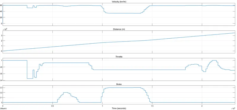
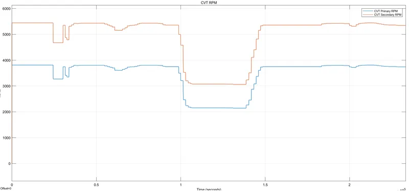
The ouput results here are inline with the inputs: instantaneous and dynamic.

C) ATV model with output of the axle mapped as an input to the CVT block.

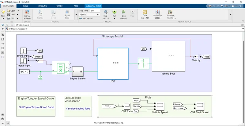
In this model the brake and throttle inputs are provided as stepped inputs. The brake is kept as 0 for the entire duration whereas the throttle input is kept as 0.3 for the first 20 seconds while for the next 80 seconds it is kept at 1. Also, the output of the vehicle body subsystem is mapped to the input of CVT subsystem and connected across the lookup table. This than becomes the input for the ‘r’ port of the variable transmission block.

Output Results

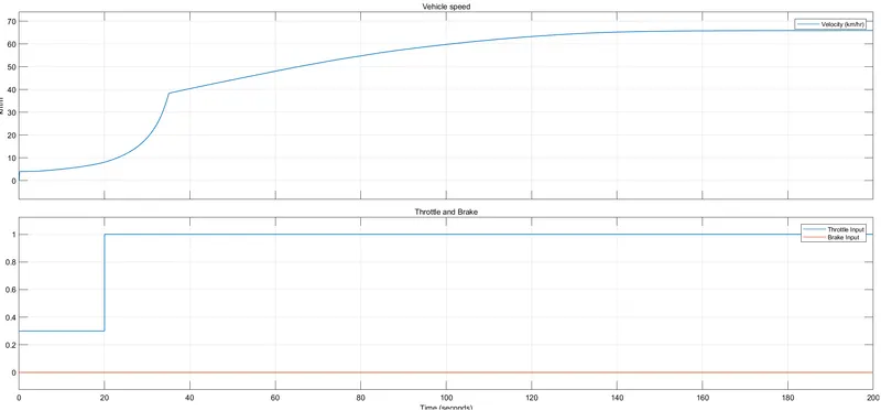
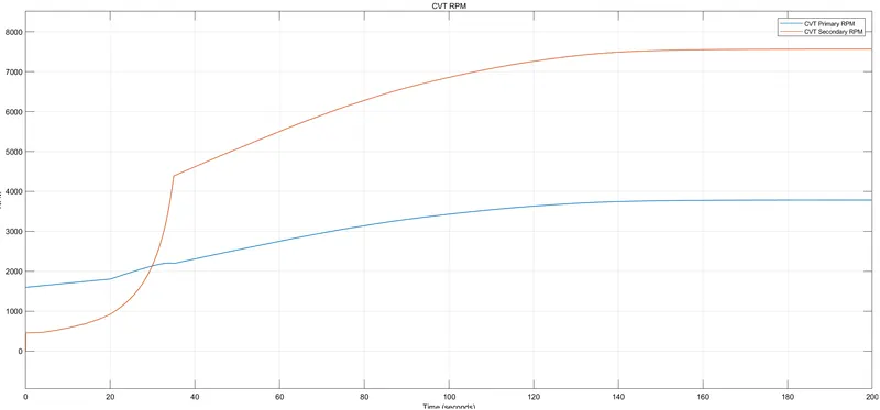
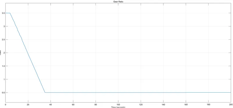
Here too the acceleration for the first 20 seconds is less as the throttle is less and after 20 seconds as the throttle increases to 1, the velocity increases continuously and attains a maximum of 65.9 kmph. The total distance travelled during this period is 2802 m. The CVT secondary RPM also increases continuously and attains a maximum of 3780 RPM.

D) ATV model with output of the axle mapped as an input to the CVT block with a dashboard facilitating knobs for dynamic inputs.

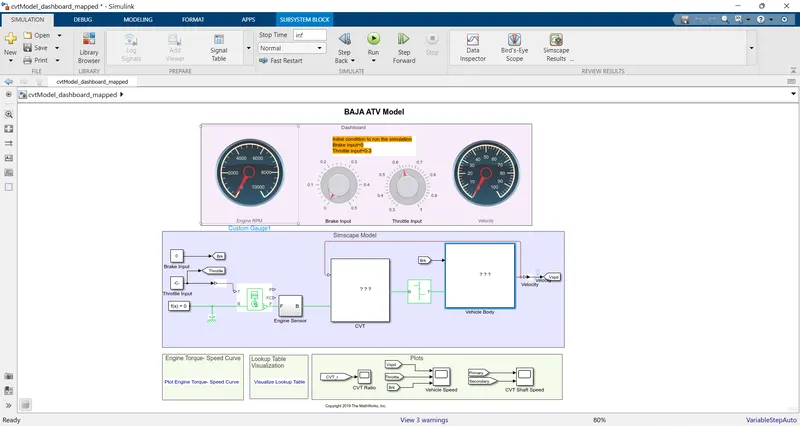
This model differs from the mapped model in that instead of the stepped inputs the inputs here are dynamic inputs provided by tuning the knobs when the simulation runs.

Output Results

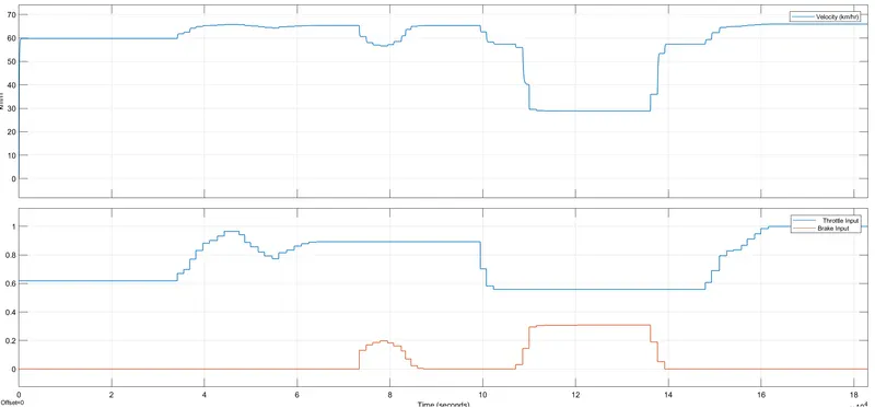
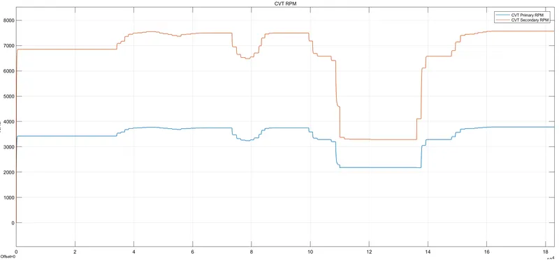
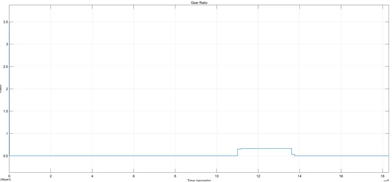
The outputs here are inline with the inputs: instantaneous and dynamic.

References:

Wikipedia

Matlab Documentation

!!!Thank You!!!