Project

Aim:

Study and research on BAJA ATV model with CVT for Open loop and Closed loop system Modelling in Simulink by using look up table.

Objectives:

• Study about BAJA ATV with CVT
• Study about CVT system
• Study about open loop, closd loop, a lookup table in for Baja ATV with CVT model
• Study and analyze the results obtained from all simulations

Theory:

In this report, we are studying Baja ATV Model with CVT. We are studying how to make the Baja ATV model in Simulink software by using differnet blocks, so for that lets first study the Baja vehicle with CVT models in details.

Baja ATV:

Baja SAE is a college design series competition run by the SAE International. Teams of students from universities all over the world design and build small off road cars. The cars have engine of same specifications.

The Goal of BAJA SAE racing is to design, build and race off road vehicles that can withstand the hardest elements of rough terrain. The vehicles used in BAJA SAE racing are often similar in appearance to dune buggies.

CVT-Continuous Variable Transmission:

A continuously variable transmission (CVT) is an automatic transmission that can change seamlessly through a continuous range of gear ratios. This contrasts with other transmissions that provide a limited number of gear ratios in fixed steps. The flexibility of a CVT with suitable control may allow the engine to operate at a constant RPM while the vehicle moves at varying speeds.

BAJA ATV with a Open loop system:

1. Baja ATV model with CVT system with fixed input to the engine and CVT by the signal builder.

2. Baja ATV model with CVT system with variable input to the engine by using variable constant which can be controlled by a knob and fixed input to CVT by the signal builder.

BAJA ATV with closed loop system:

1. Baja ATV model with CVT system fixed input to the engine through the step block and input to CVT ratio is selected based on vehicle speed with the help of loop up table as a close loop system

2. Baja ATV model with CVT system with variable input to engine controlled by a knob and input to CVT ratio is selected based on vehicle speed with the help of look up table as a close loop system.

Blocks Used:

1. Signal builder
2. Generic Engine: Speed power and Speed torque parameters are provided. A throttle physical signal inout specifies the normalised engine torque. Optional dynamic parametrs include crankshaft inertia and response time lag.
3. Ideal rotational motion sensor: R port-Mechanical rotational conserving port associated with the sensor positive probe. C port- Mechanical rotational conserving port associated with the negative porbe (refernce). W port-PS output for angular velocity. A-PS output for angular dispalcement.
4. Variable ratio Transmission: It represents a gearboc that dynamically transfer motion and torque between 2 connected driveshafts axes, base and follower. B port- It is a rotational port representing the primary pulley. F port - it is a rotational conserving port representing the secondary pulley of CVT. R port- We specify the gear ratio as a function of timeat the physical signal input port "R".
5. Simple Gear box:
6. Vehicle Body: It represents a 2 axle vehicle body in longitudnal motion. The block accounts for Body mass, Aerodynamic drag, road incline and weight distribution between axles due to accelaration and road profile.
7. Tire (magic formula) : It models a tire with longitudnal behaviour given by mafic formula, an emperical equation based on 4 fitting coefficients. The block can model tire dynamics under constant and variable pavement conditions. N port - PS inout port associated with the normal force acting on the tire. Force is positive if it acts downwards on the tire, pressing it against the pavement. S port_ Phycial singal output port associated the the relative slip between the tire and road. A port - Mechanical rotational port associated with the axle that the tire sits on. H port- Mechanical translational port associated with the wheel hub that transmits the thrust generated by the tire to the remainder of the vehicle.
8. Double shoe brake: It represnts a frictional brake t=with 2 pivoted rigid shoes that pres against a rotating drum to produce a braking action. F port - PS input port associated with the rotating drum shaft.

1.a) Baja ATV model with CVT system with fixed input to the engine and CVT by Signal builder.

Simulink model:

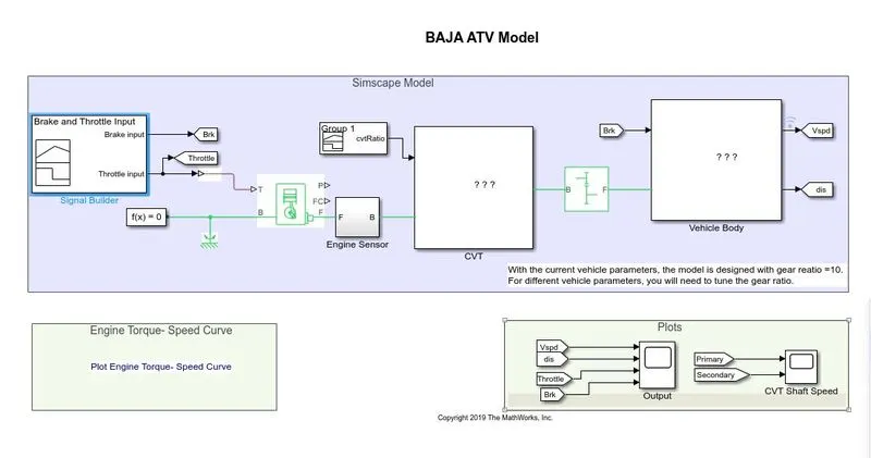
Model Explaination:

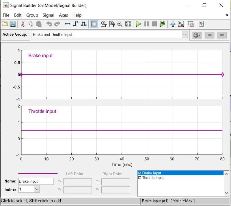
1. Give input to the engine with the help of signal builder. We have one input to the engine ehich is throttle, in sigal builder we are giving constant throttle of half press on throttle for 80 sec. As we are not considering the braking condition for the vehicle we kept input brake zero. the inputs in the signal builder are shown below:
   
2. Define the inputs for the engine, for representing the engine we are using the Generic engine block which is available in simulink we have to give some parameters of the engine like Speed vector, Torqur vector, Inertia, Ideal RPM which is shown in the below figure:
   
   
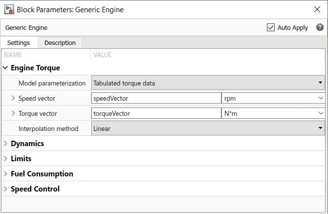
   The Speed vector and torque vector are the variables defined in the Matlab workspace, the data fro speed and torque vector is taken from the graph which is as shown in below diagram using the grabit program.
3. The output of the engine i.e crankshaft, is connected to the ideal rotational motion sensor to measure the RPM of the engine and plot the graph by using scope block. O/P of the engine is also connected to the input shaft(base) of the Varable transmission ratio which ascts as a CVT.
4. 
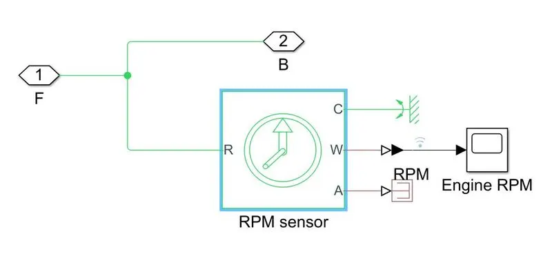
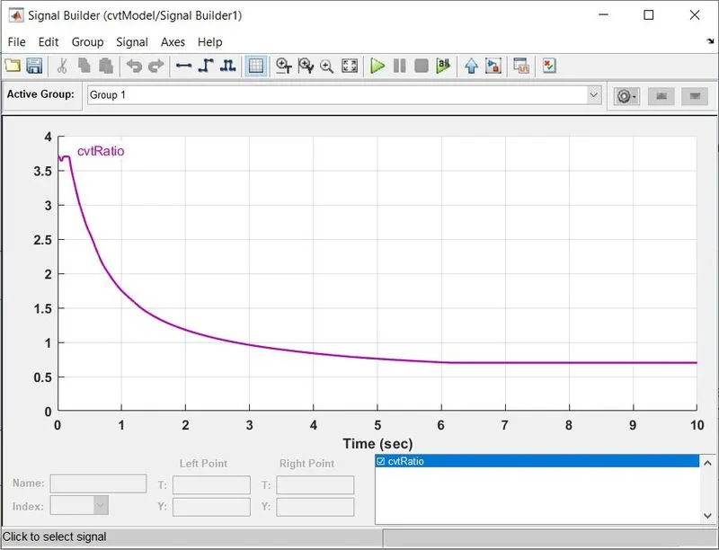
5. Output from the engine is connected to the Input shaft or the primary shadt of the CVT. In CVT there is a contuinuous change in gear ratio. So for that we have to give input CVT ratio for the given range which depends on CVT model. So the input for variable ratio transmission block to act as a CVT is given with the help of signal builder to the port R as shown in below figure.
   For inertia block, m1 and m2 are 3.5kg and 3.2kg which are defined in the matlab workspace. We have connected the idel rotational motion sensor to the input and output shaft, i.e. primary and secondary pulley of the CVT to measure the RPM of both pulleies.
6. The ouput of CVT, i.e secondary pulley is connected to the input of the simple gear box which is having a gear ratio of 10.
   
7. Last step is to connect the output of the gearbox shaft to the rear wheel of Baja ATV for which we have to make the Baja ATV model:
   
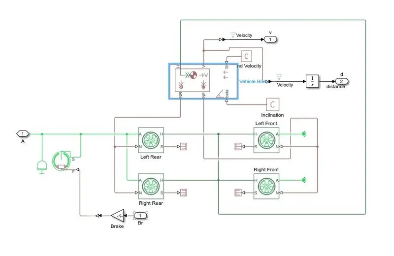
   We are considering a rear wheel drive system for Baj ATV model so we have connected the Output of the gearbox to rear wheels only. we are also connecting double rear wheel and front wheel and other parameters of the vehicle we are using vehicle body block which is available in Simulink. Input parameters are: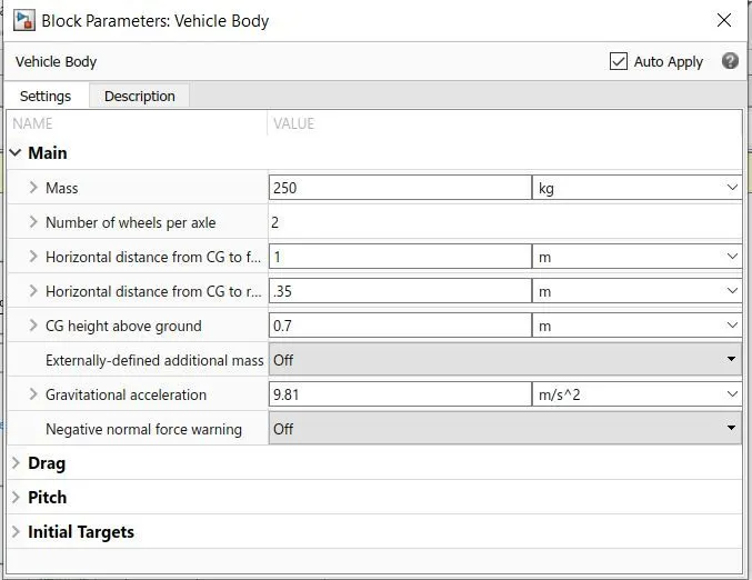
   
8. To plot the outputs we are using goto and from blocks to connect the scope.

Outputs:

Graph for the vehicle speed and distance for given value of throttle and brake:

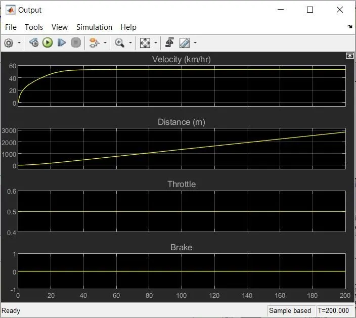
Result: As we can see that when we press the throttle to 0.5 the vehicle speed increases to its correspoding value with corresponding distance.

Graph for primary and secondary rpm of the CVT:

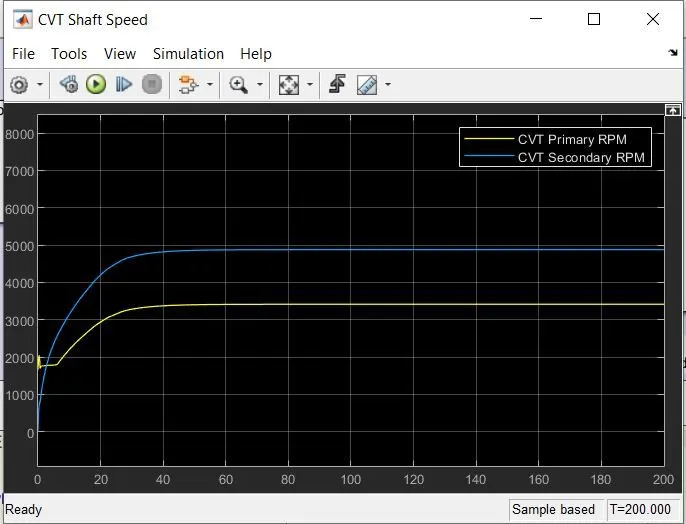
Result: As we can see that as primary pulley RPM increase the corresponding secondary pullet RPM increases wrt the given CVT ratios.

Graph for Engine RPM:

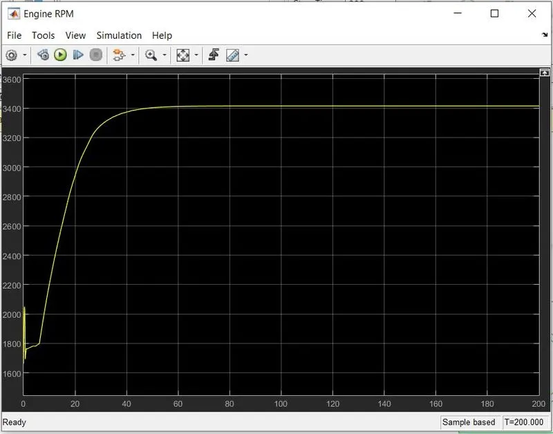
From the above four graphs we can say that as we press the throttle to 0.5 the engine attains its corresponding rpm, first the rp decreases to get the required torque to move the vehicle then it increases wrt time. now next this engine rpm is transferred to the seondary pulley with the help of primary pulley. For gien vehicle rpm the CVT ratios are selected from signal builder.

1. b) Baja ATV model with the CVT system with variable input to the engine by using variable constant which can be conroled by a knob and fixed input to CVT by singal builder:

Simulink Model: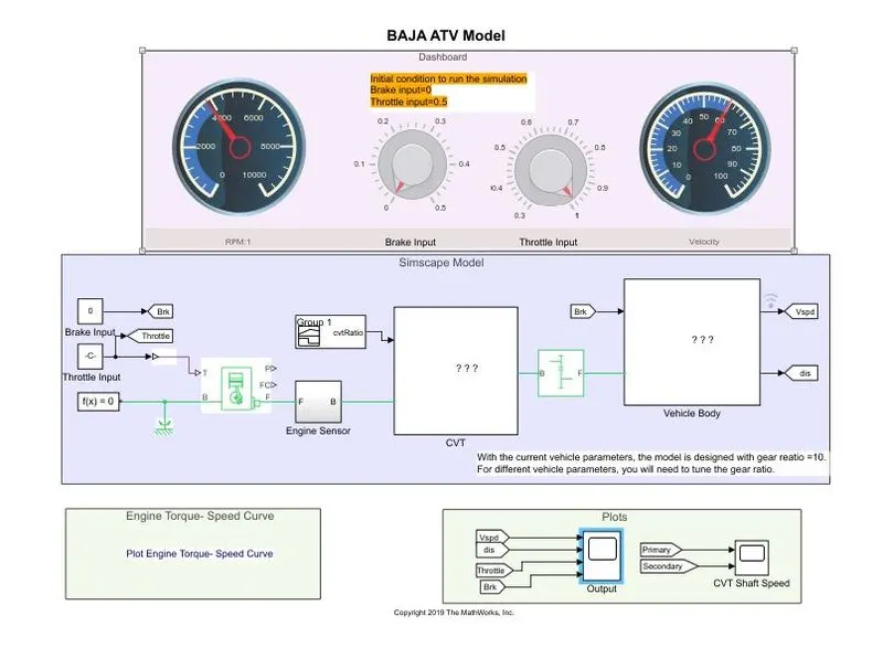

Model explination:

This model is similar to model 1.a but the difference is only the type of input values of the throttle and brake with the help of nobs.

In this model the simulation run time is kept as inf so that we can change the values of the throttle and brake with the help of the input parameters.

We also have 2 cicular gauges which are connected to measure the rpm of the engine and velocity of the vehicle as shown in above daigram.

Results:

Graph for change in vehicle speed and distance for given input of throttle and brake.

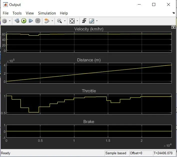
As we change the input throttle values with the help of the knob the corresponding vehicle speed increases or decreases.

Graph for primary and secondary pulley RPM of CVT:

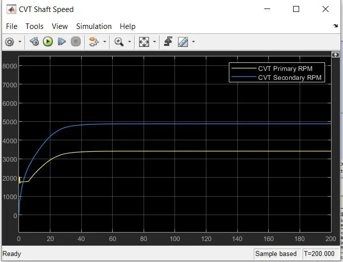
The secondary pulley RPM increases or decreases wrt to the primary pullet RPM i.e. te rpm of engine and corresponding CVT ratios.

Graph for Engine RPM:

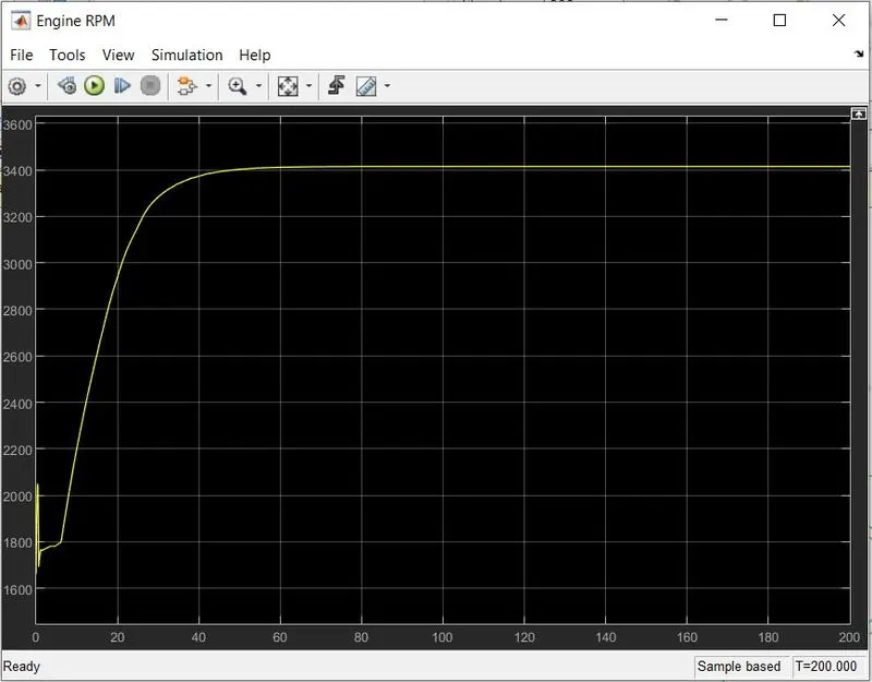
The rpm of the engine changes according to the throttle input.

2. a) Baja ATV model with CVT system with fixed input to the engine through the step block and input to CVT ratio is selected based on vehicle speed with the help of look up table as a closed loop system.

Simulink model:

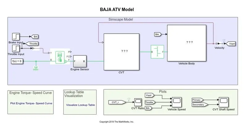
Explaination for Simulink model:

1. In this model we are giving input to the engine with the help of step blocks. As we know that the we are considering only accelarating conditions so we are keeping the braking condition zero throughout the simulation. The input to the engine with the help of shown values

Throttle Input:

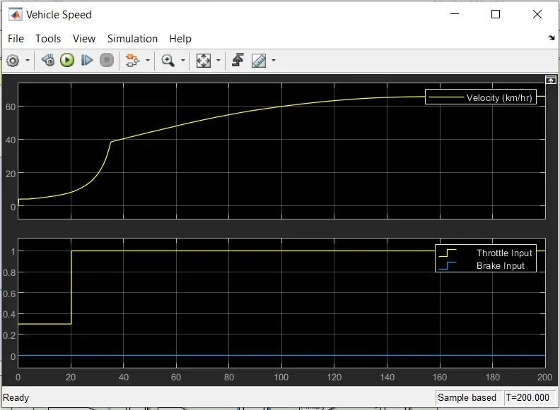
As per these value throttle will be pressed 0.3 for 0 to 20 sec and at a 20 sec it will increase to the final value which is 1 for the rest of the simulation time.

Brake Input: Through out the simulation time the brake input is 0.

2. The output of the throttle and brake is connected to the scope block and Generic engine input. Paramters for generic engine are:

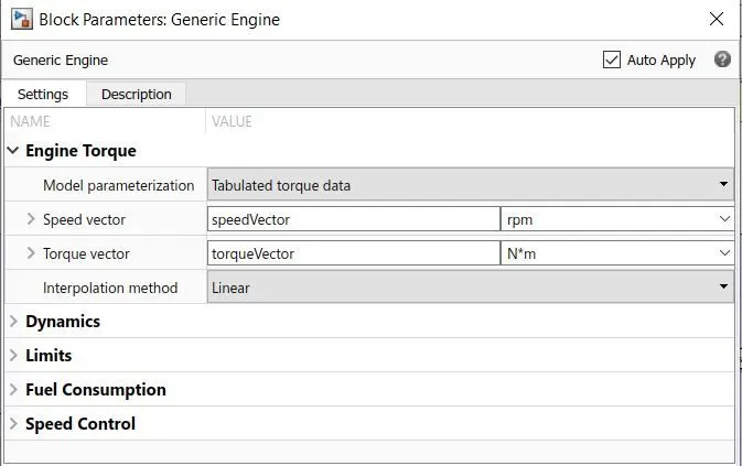
The speed vector and torque vector are variables defined in Matlab workspace form the below graph data points with the help of Grab it program.

3. The output of the engine is connected to the ideal rotational motion sensor to get the RPM of the engine and next the output of the engine is connected to the input shaft of the variable ratio transmission block i.e the primary pulley of CVT. We are using Look up table for variable ratios.

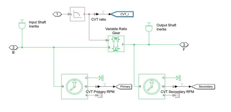
Lookup Table:

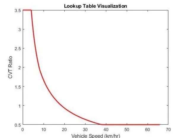
We are selecting the CVT ratios according to the velocity of the vehicle which is connected to the input of the look up table from the output of the vehicle model. In the lookup table for input cwe are taking CVT Ratios so wehn we run the simulation CVT changes its ratio according to the vehicle velocity of the vehicle body.

As we can see this model is the same as 1.a model but the only differnce is that we have connected 'To workspace' blocks at the output of the CVT ratio graph and the output of the vehicle speed at the vehicle body as shown in the above diagram marked with the yellow marker. These blocks are connected to collect data to the workspace so we can use that in the look up table.

Now the output of the lookup table is connected to the GOTO block to get the graph of the output CVT ratios in graph format. We can also do lookup table parametes visualization by writing the below program in Matlab.

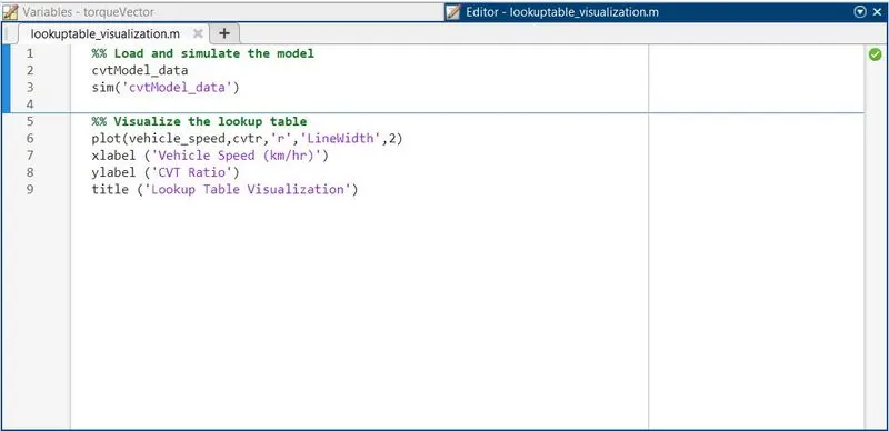
We are using a sim command to open and run the above Simulink model, after completion of the simulink, the data to plot the graph to do visualization of the lookup table.

Now we have connected the output of the engine to the input of the variable ratio transmission and the output shaft of the variable ratio transmission is connected to the inout of the gearbox. Accross these two shafts, we have connected the inertia blocks to give the inertia and also connected to the ideal rotational motion sensor block to measure the RPM of the primary and seconday pulley.

4. Now the output of the secondary pulley is connected to the input shaft of the gearbpx. We are using a gearbox with a gear ratio of 12 in this simulation.

5. Next the output of the gearbox is connected to the both rear wheels of the Baja ATV because we are considering rear wheel drive system and also we have connected double shoe brake to the rear wheel as shown in diagram:

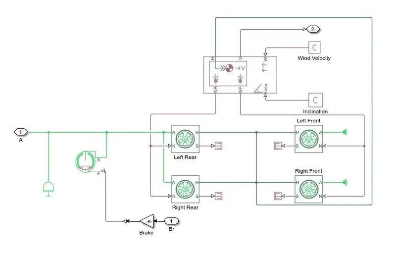
The front wheel(NF) and rear wheel(NR) are defined by using vehicle body block. The all wheels are connected to the H-port to give only horizontal motion to the wheels. The output port of vehicle body which is the soeed is connected to the GoTo block to connect it to scope by using from block to plot the graph. To plot the graph use Scope block.

Results:

Graph for vehicle speed wrt throttle and brake values:

In this graph the speed increases continuously according to the throttle input and one the throttle input reaches to maximum value of 1 the speed increases to its maximum value

Graph for primary and secondary pulley of CVT:

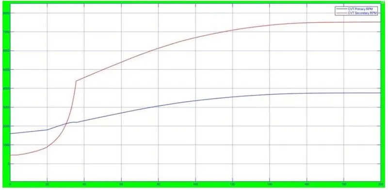
The secondary pulley rpm is low for starting time compared to the primary pulley rpm because to get initial torque required to move the vehicle. As we are giving input to the CVT wrt vehicle spped by look up table so when the input speed as low it select the required CVT ratio to get required secondary pulley rpm.

Graph for engine rpm:

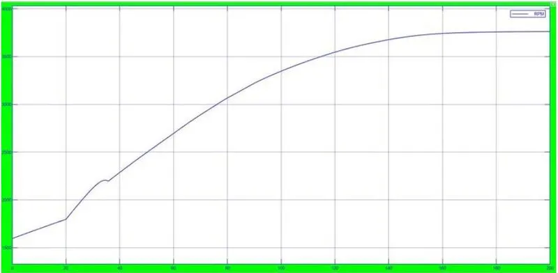
As we know for 1st 20sec the throttle input is 0.3 so the engine rpm is low once the engine input throttle jumps to 1 values the engine rpm increases rapidly wrt time.

Graph for CVT ratios from lookup table:

2.b) Baja ATV model with CVT system with variable input to the engine which can be controlled by knob and inout to CVT ratio is selected based on vehicle speed with the help of lookup table as a close loop system.

Simulink Model:

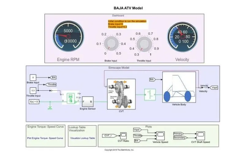
The model is same as 2.a but the only differnce is type of input we are giving to the engine block. i.e real time simulator.

In this model we have connected throttle and brake tothe engine with the help of constant blocks which are connected to the knob.

The throttle knob can be varied to the range of 0.3 to 1 and brake knob can be varied to the rage of 0.3 to 1 and brake knob can be varied tothe range of the 0 to 0.5.

We also connected the engine rpm and the vehicle speed.

Results:

As the throttle input to the engine increases or decreases the corresponding vehicle speed increases or decreases concerning time.

For the initial simulation time the CVT ratio is high to provide the required torque to the engine once the speed of the vehicle increases the CVT ratio goes on decreasing.

The enigne rpm increases or decreases accordnig to the input throttle values.

For the inital time the secondary pullet rpm increases and after some time it changes according to the primary pulley rpm and according to the vehicle speed to select the correct CVT reduction ratio from the lookup table.

Conclusion:

From this case study we learned how to make Baja ATV model with CVT system using Simulink blocks, Next we learned how we can use lookup table sto add more realistic conditions for Baja ATV model with CVT system from the above graph we can also adjust the gear ratio or CVT rario for different conditions instead of trying to do on real model which takes more time. As we can also plots for graph of different outputs we can adjust the ratios of the both CVT and gearbox, we can get the required tuning for the required track conditions.