Project
::: BAJA ALL-TERRAIN (ATV) MODEL WITH CONTINUOUSLY VARIABLE TRANSMISSIOM(CVT)::
>> Aim::
carry out a system-level simulation of BAJA all terrian vehicle with an combination of continuously variable transmission (CVT) system.
> OBJECTIVES:
1) To prepare a technical report explaning the moodel properties and comment on the output results.
2) Explain the function of the subsystems and blocks for preparaing the model
ALL TERRAIN VEHICLE (ATV):
An all-terrain vehicle (ATV), also known as a light utility vehicle (LUV),a quad bike, or simply a quad, as defined by the American National Standards (ANSI) is a vehicle that travels on low-pressure tires, with a seat that is straddled by the operator, along with handlebars for steering control.
As the name implies, it is designed to handle a wider variety of terrain than most other vehicles.
BAJA ATV (SAE):
> The Baja SAE is an intercollegiate engineering design competition for undergraduate and graduate engineering students.
>The object of the competition is to simulate real-world engineering design projects and their related challenges.Is organized globally by the 'society of Automotive Engineers,(SAE) in USA.
> In 1976 at university of carolina firstly organized.
> BAJA is basically an ATV competition where students get to design and develop their own ATV keeping in mind various considerations of design as well as safety. An ATV is designed in order to run on various terrains such as soil, Gravel, pebbles.
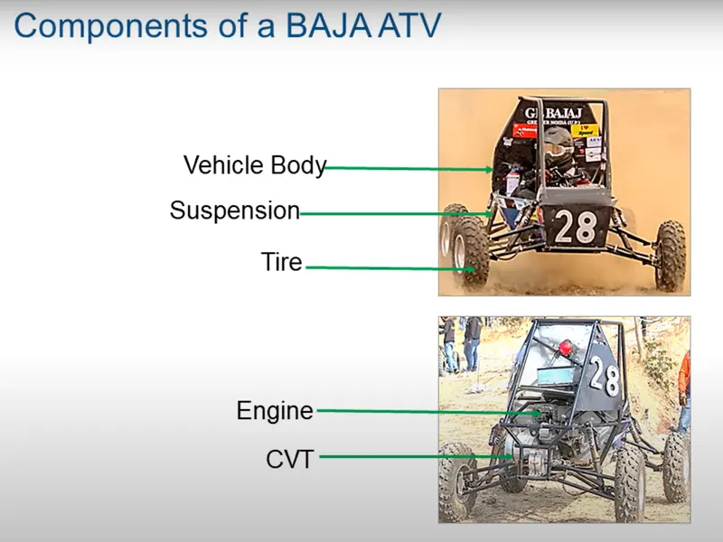
>Components of BAJA ATV:
>> BAJA ALL-TERRAIN VEHICLE MODEL:
> STAGES OF WORK FLOW:
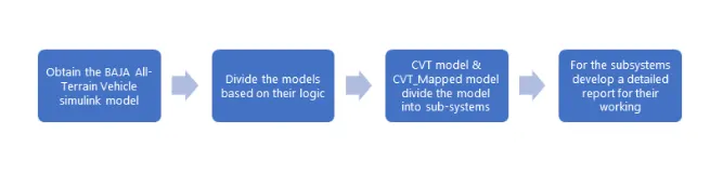
- Obtain the BAJA ALL -Terrain vehicle simulink mode
- Divide the models based on their logic
- CVT model and CVT_Mapped model divide the model into sub-systems
- For the subsytems develop a detailed report for their working
>This submission contains a set of models created with Simulink, Simscape, and Simscape Driveline.
>More specifically, the file contained includes BAJA ATV model with Continuously Variable Transmission(CVT).
>These models show how to build an ATV with CVT which is mostly used in BAJA competitions. Simscape and Simscape Driveline have been used to complete the system.
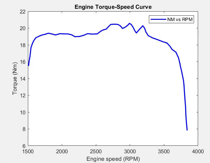
>The engine data used in the model is provided as an image which shows the Engine Speed (RPM) Vs Torque curve.
> CVT::
>continuously variable transmission (CVT) is an automatic transmission that can change seamlessly through a continuous range of gear ratios.
>This contrasts with other transmissions that provide a limited number of gear ratios in fixed steps. The flexibility of a CVT with suitable control may allow the engine to operate at a constant RPM while the vehicle moves at varying speeds.
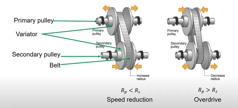
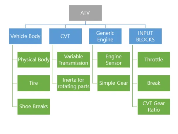
>components of the system:
>> BLOCKS Requried:
1) signal Builder: The Signal Builder block allows you to create interchangeable groups of piecewise linear signal sources and use them in a model. You can quickly switch the signal groups into and out of a model to facilitate testing.
>In the Signal Builder window, create signals and define the output waveforms.
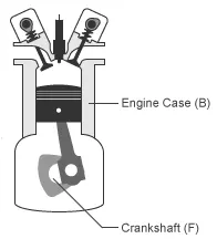
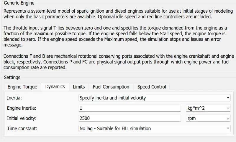
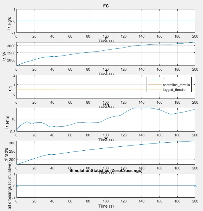
2) Generic Engine: Represents a system-level model of spark-ignition and diesel engines suitable for use at initial stages of modeling when only the basic parameters are available. Optional idle speed and red line controllers are included.
Generic Engine
>The throttle input signal T lies between zero and one and specifies the torque demanded from the engine as a fraction of the maximum possible torque.
>If the engine speed falls below the Stall speed, the engine torque is blended to zero. If the engine speed exceeds the Maximum speed, the simulation stops and issues an error message.
>Connections F and B are mechanical rotational conserving ports associated with the engine crankshaft and engine block, respectively. Connections P and FC are physical signal output ports through which engine power and fuel consumption rate are reported.
3) Gear box: Represents a fixed-ratio gear or gear box. No inertia or compliance is modeled in this block. You can optionally include gear meshing, backlash, and viscous bearing losses.
4) Goto: Send signals to From blocks that have the specified tag. If tag visibility is 'scoped', then a Goto Tag Visibility block must be used to define the visibility of the tag.
5) Subsystems: A Subsystem block contains a subset of blocks within a model or system:
>> SIMULINK BLOCK DIAGRAM ::
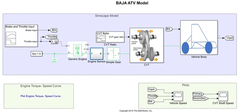
> Required inputs to the system:
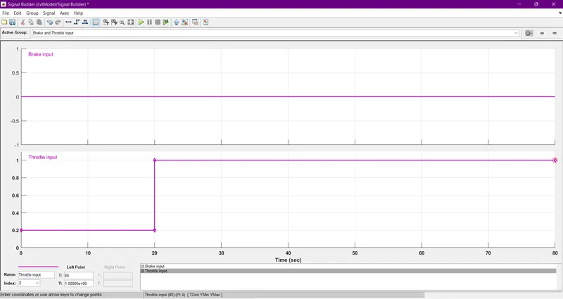
> The signals are given to the system through the signal builder
> one signal for the brake input and another for the throttle input.
>observed that currently there is no break point provided to the system and aconstant throttle is provided whcih change after 20sec into the simulation.
> Engine setting:
> For this particular model we have specified the initial inertia of 1kg*m^2 ,and initial velocity of 2000 rpm.
> limit span of 100 rpm as speed threshold.
Engine sensor
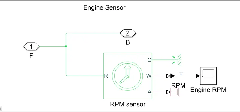
> The block represents an ideal mechanical rotational motion sensor,that is ,a device that converts an across variable measured b/w two mechanical rotational nodes into a control signal proportational to angular velocity or angle.
> The sensor is ideal since it does not account for inertia,friction,delays,enery consumption,and so on.
> connections R an C are mechanical rotational conserving ports and connections W and A are physical signal output ports for velocity and angular displcement.
PLOT: Primary RPM
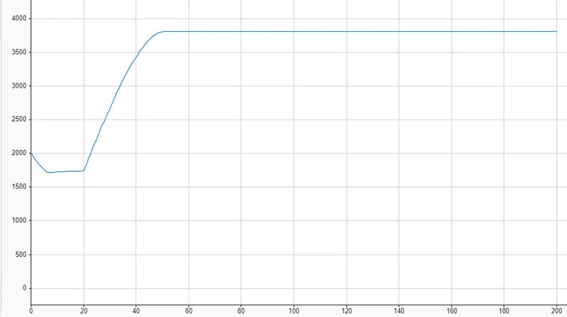
> Here we observe that the rpm falls from 2000 to a significant portion and then gradually picks up and rise after 20 sec Then after at 40sec rises and becomes constant. as shows in graph.
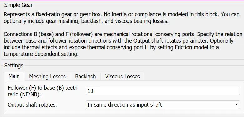
simple Gear : Represents a fixed-ratio gear or gear box. No inertia or compliance is modeled in this block. You can optionally include gear meshing, backlash, and viscous bearing losses.
>Connections B (base) and F (follower) are mechanical rotational conserving ports. Specify the relation between base and follower rotation directions with the Output shaft rotates parameter. Optionally include thermal effects and expose thermal conserving port H by setting Friction model to a temperature-dependent setting.
> Here Follower (F) to base (B) teeth ratio (NF/NB)=10
> CVT (continously variable transmission) MODEL:
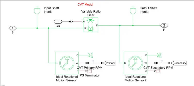
> The CVT Controller block implements a push belt continuously variable transmission (CVT) controller. The block uses standard pulley and geometric equations to calculate the kinematic setpoints for the CVT variator. You can use the block to control a CVT.
> Here the two inertia blocks represents the primary pulley and the output shaft inertia represents the secondary pulley.
>variable gear ratio:Represents a variable ratio gearbox such as implemented by mechanical belt CVT, electric, or hydraulic transmissions. The physical signal input r defines the ratio of input to output angular shaft velocities.
>Connections B (base) and F (follower) are mechanical rotational conserving ports. Specify the relation between base and follower rotation directions with the Output shaft rotates parameter.
Input to the CVT system:
> Here input is provided by the signal bulider
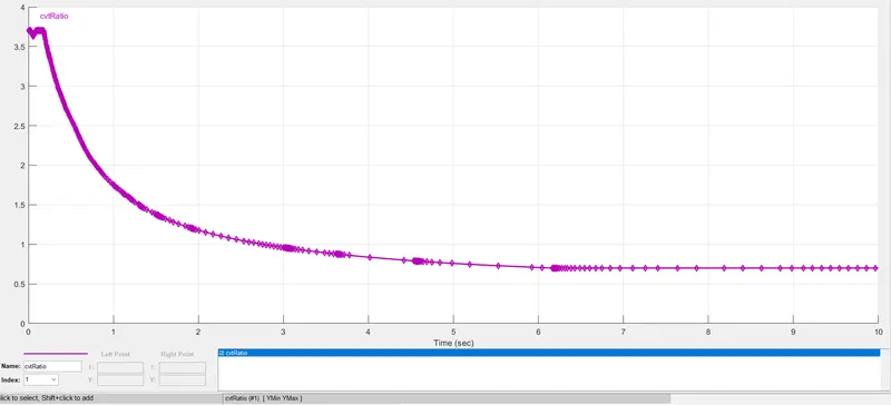
> From the graph we observed that the given gear ratio as 10 and which varies by the y value .
> Vehicle Body Subsystem:
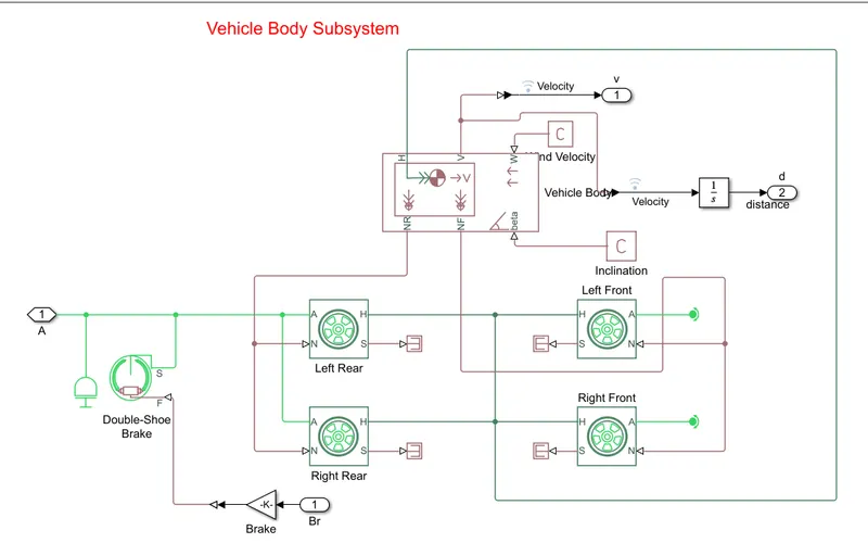
>Vehicle Body:Represents a two-axle vehicle body in longitudinal motion. The block accounts for body mass, aerodynamic drag, road incline, and weight distribution between axles due to acceleration and road profile.
>The vehicle can have the same or a different number of wheels on each axle. Optionally include pitch and suspension dynamics or additional variable mass and inertia. The vehicle does not move vertically relative to the ground.
>Connection H is the mechanical translational conserving port associated with the horizontal motion of the vehicle body. The resulting traction motion developed by tires should be connected to this port.
>Connections V, NF, and NR are physical signal output ports for vehicle velocity and front and rear normal wheel forces, respectively. Wheel forces are considered positive if acting downwards.
> Connections W and beta are physical signal input ports corresponding to headwind speed and road inclination angle, respectively. If variable mass is modeled, the physical signal input ports CG and M are exposed. CG accepts a two- element vector representing the x and y distance offsets from vehicle CG to additional load mass CG. M represents the additional mass.
>If both variable mass and pitch dynamics are included, the physical signal port J accepts the inertia of the additional mass about its own CG.
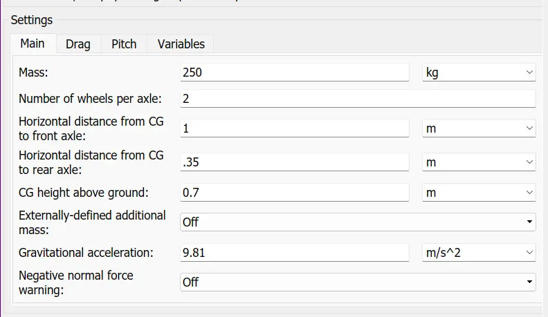
Vehicle Body Settings:
> Double Brake Shoe: Represents a brake arranged as two pivoted rigid shoes symmetrically installed inside or outside a drum and operated by one actuator. The actuator force causes the shoes to exert a friction torque on a shaft connected to the drum.
F — Actuating force
S — Drum shaft rotation
> Wheel (Tire) :Represents the longitudinal behavior of a highway tire characterized by the tire Magic Formula.
>The block is built from Tire-Road Interaction (Magic Formula) and Simscape Foundation Library Wheel and Axle blocks. Optionally, the effects of tire inertia, stiffness, and damping can be included.
>Here
N — Normal force
S — Slip
A — Axle
H — Hub
>The Tire (Magic Formula) block assumes longitudinal motion only and includes no camber, turning, or lateral motion.
>Tire compliance implies a time lag in the tire response to the forces on it. Time lag simulation increases model fidelity but reduces simulation performance.
OUTPUTS
>workspace:
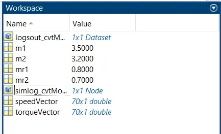
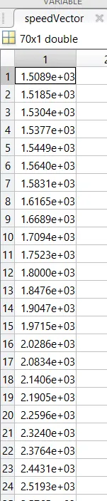
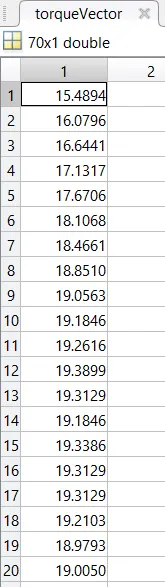
> The Engine will generate the output rpm which can be taken from the crankshaft output.This speed will be given to the ideal rotational motion sensor to sense the output rpm.
> Then the output speed of the engine is given to CVT to reduce the speed.The CVT ratio is provided to the variable transimmision CVT block through signal builder..
>CVT rpm:
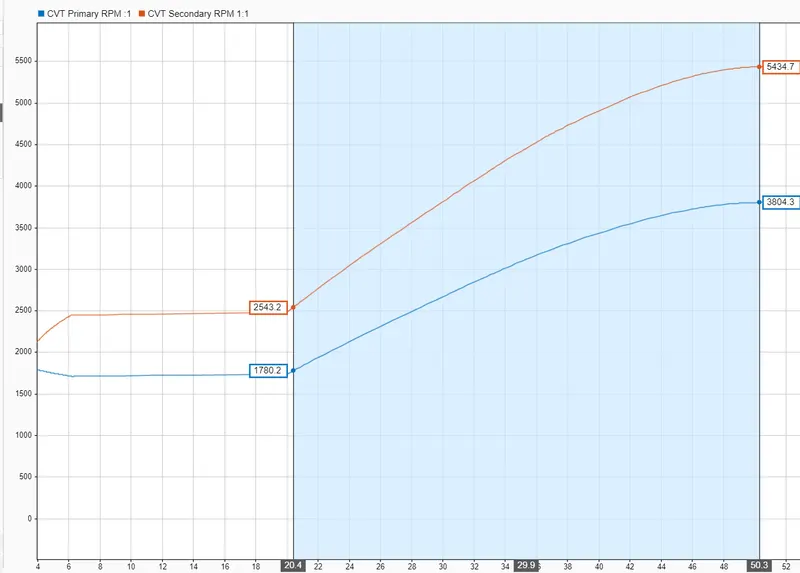
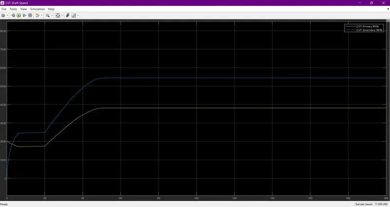
> We can observe that the secondary pulley is rotating at a lower rpm than the primary pulley and hence we can see that this arrangemnet is to supply torque to the engine.
> Here the maximum RPM is nearly about 6000 rpm and cvt ratio is 1:10
> Engine Torque speed:
> velocity,distance,throttle,brake plots:
> shaft primary and secondary plots:
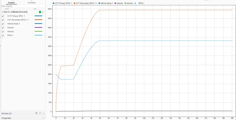
> plot:
> here we can observe the different plots of cvt rpms,velocities.
::: BAJA ATV MODEL WITH DASHBORAD:::
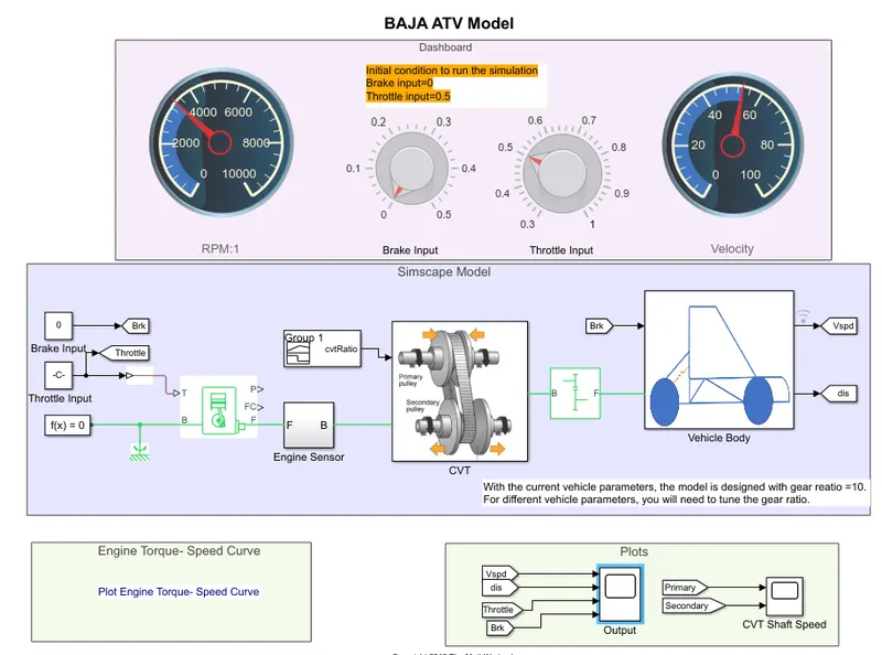
>> Main Model:
DASHBOARD:
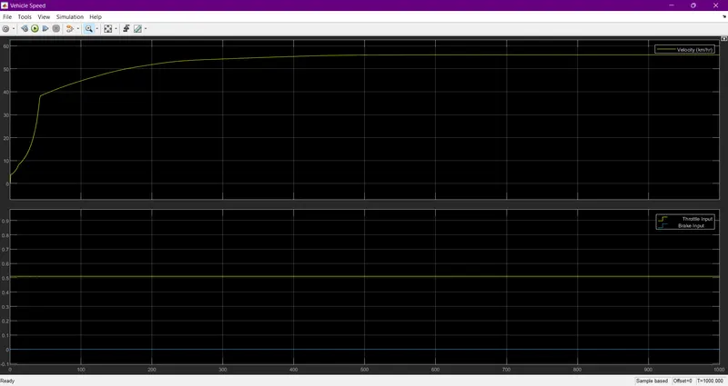
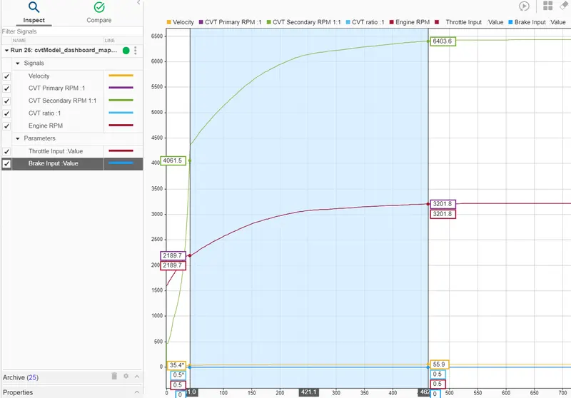
> Here running an simulation at Throttle input=0.5 and Brake input =0.
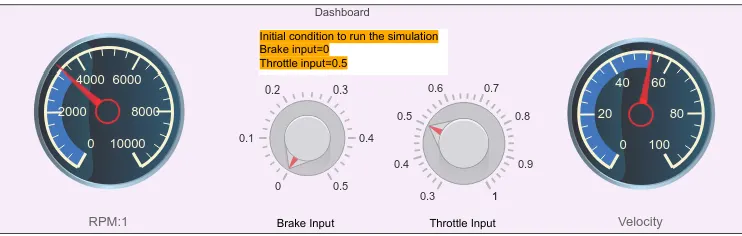
>Circular Gauge block displays the value of the connected signal on a circular gauge that you can design to look like a gauge in a real system.
The Circular Gauge block displays the instantaneous value of the connected signal throughout simulation. You can modify the range and tick values on the Circular Gauge block to fit your data. Use the Circular Gauge block with other dashboard blocks to build an interactive dashboard of controls and indicators for your model.
> Knob block tunes the value of the connected block parameter to during simulation. For example, you can connect the Knob block to a Gain block in your model and adjust its value during simulation. You can modify the range of the Knob block's scale to fit your data. Use the Knob block with other Dashboard blocks to create an interactive dashboard to control your model.

>> FLOW PROCESS:
The model work flow process is as same as the process of 'BAJA ATV model without Dashboard' but the throttle and brake inputs are controlled by the user with the knob.we are also replacing signal bulider with two seperate constant blocks for the throttle and brake.
OUTPUTS:
> Engine Torque speed:
>CVT shaft speed:
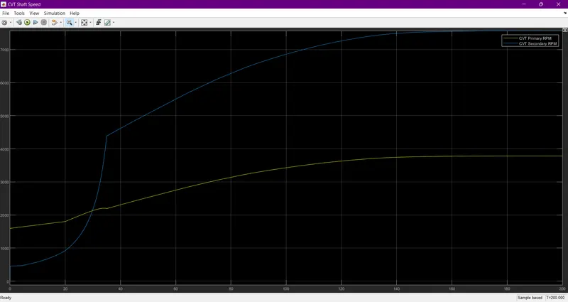
> Here from the above plot we observed that the primary pulley and secondary puley are rasise upto as certain rpm then after becomes constant and runs at an time span of 200sec.
> velocity plot:
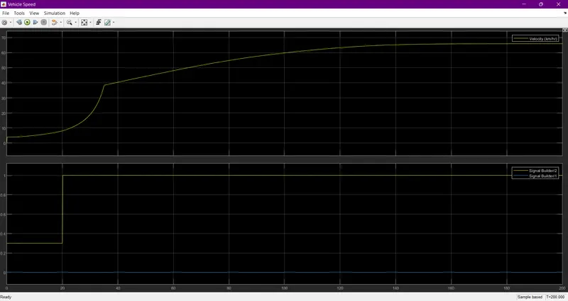
> velocity of body,RPM of CVT plots:
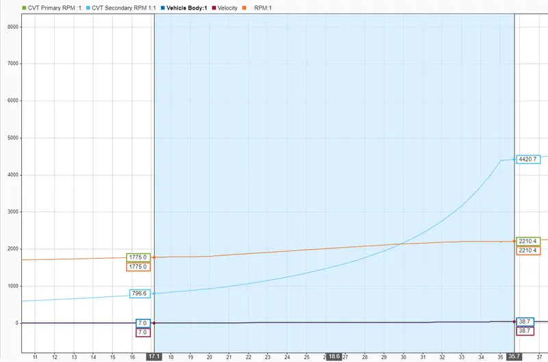
> From the above plot the primary,secondary rpms are becomes constant at an certain rpm.
> velocity,distance,throttle,brake plots:
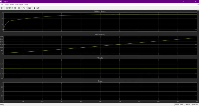
::: BAJA ATV MODEL - MAPPED LOOKUP TABLE WITH DASHBOARD:::
>> Main Model:
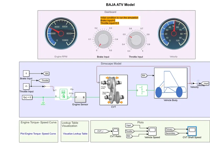
> Here we are connecting the cvt directly to the vehicle body output by this body provide an input to the CVT primary pulley.speed varies constantly by this.
> Running the dashboard at Throttle as 0.5 and brake input as 0
> CVT Model:
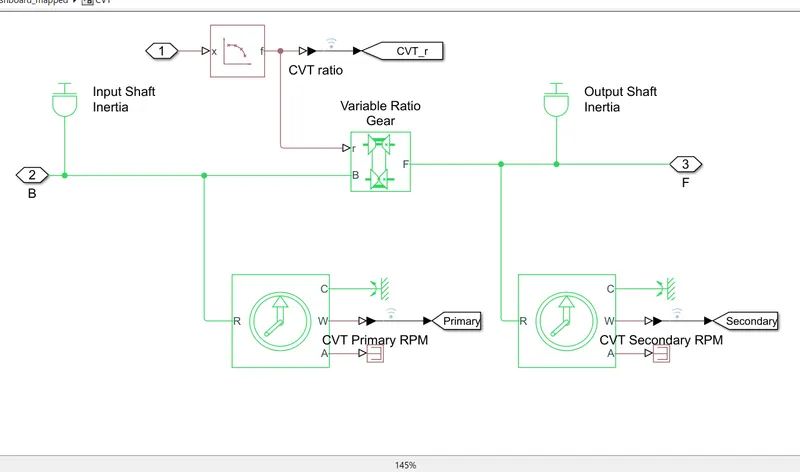
LOOK UP Table:
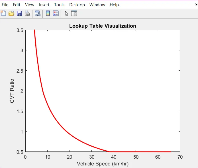
>The PS Lookup Table (1D) block computes an approximation to some function f=f(x) given data vectors x and f. Both the input and the output are physical signals.
>The length of the x and f data vectors provided to this block must match. Also, the x data vector must be strictly monotonic, either increasing or decrease.
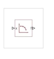
symbols:
x — Input query point, or a row or column vector of query points, along the x-axis, untyped
f — Output function value, untyped
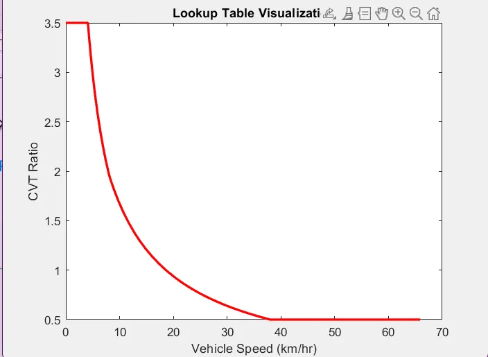
> define the lookup table by specifying the Table grid vector parameter as a 1-by-n vector (x data vector) and the Table values parameter as a 1-by-n vector (f data vector). The block generates output based on the input values using the selected interpolation and extrapolation methods. You have a choice of two interpolation methods and two extrapolation methods. You also have an option for the block to issue an error if the input signal value is outside the table grid vector range.
>> FLOW PROCESS:
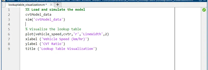
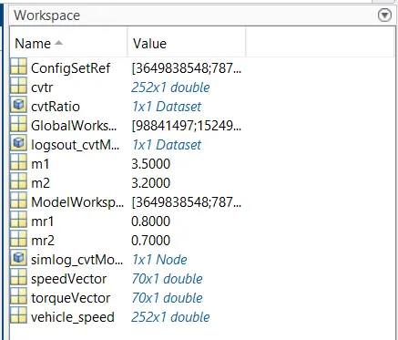
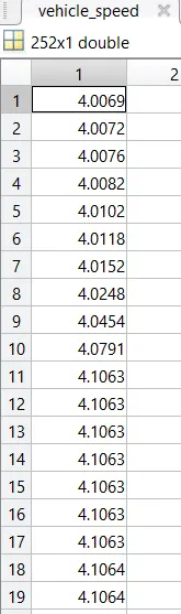
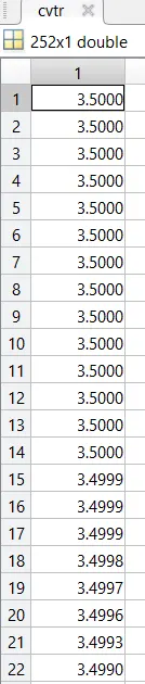
The workflow process is as same as the process of 'BAJA ATV Model with dashboard' .The small addition is here the CVT ratio and vehicle speed are extracted by using 'workspace'
>OUTPUT:
> By running the simulation at an time span of 200sec we are getting different outputs.
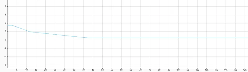
>CVT RATIO PLOT:
> For 200 sec time the CVT ratio plot as shown below;
> CVT output:
> vehicle speed:
> Generic Engine:
>Dashboard result:
::: BAJA ATV MODEL- MAPPED LOOK UP TBALE WITHOUT DASHBOARD:::
>> MAIN MODEL:
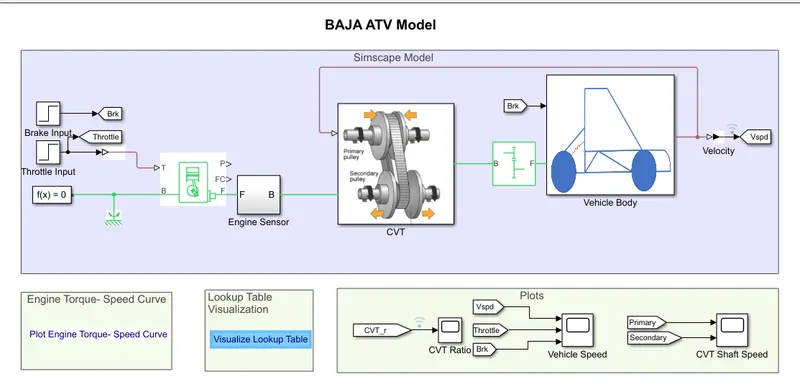
> Here brake and throttle inputs are provided by an constants.
> FLOW PROCESS:
The flow process is as same as 'BAJA ATV mapped model with dashboard' .
> Look up Table:
>The PS Lookup Table (1D) block computes an approximation to some function f=f(x) given data vectors x and f. Both the input and the output are physical signals.
>The length of the x and f data vectors provided to this block must match. Also, the x data vector must be strictly monotonic, either increasing or decrease.
>>OUTPUTS:
>CVT ratio:
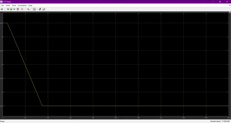
> Here the speed is controlled by the variable CVT ratios and the controlled output speed is inputted to the vehicle axle.
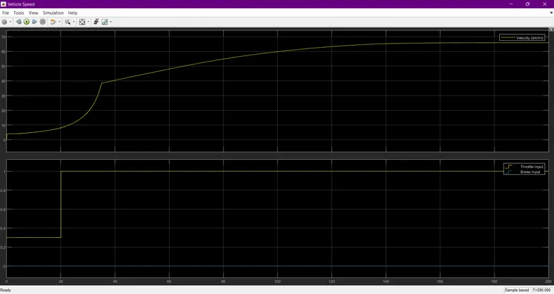
> vehicle speed:
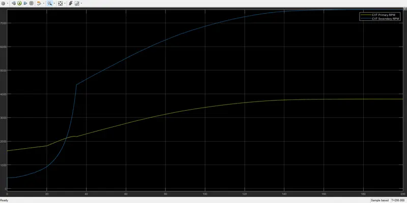
> CVT Shaft speed:
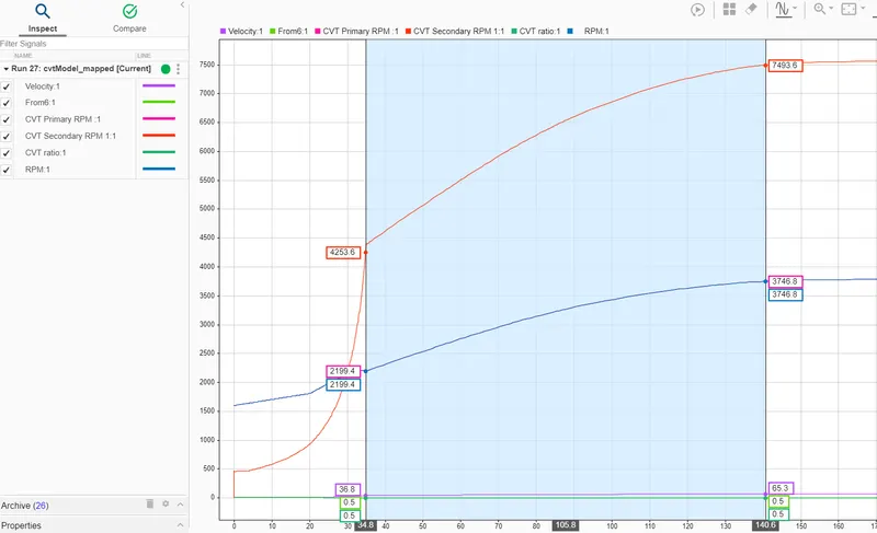
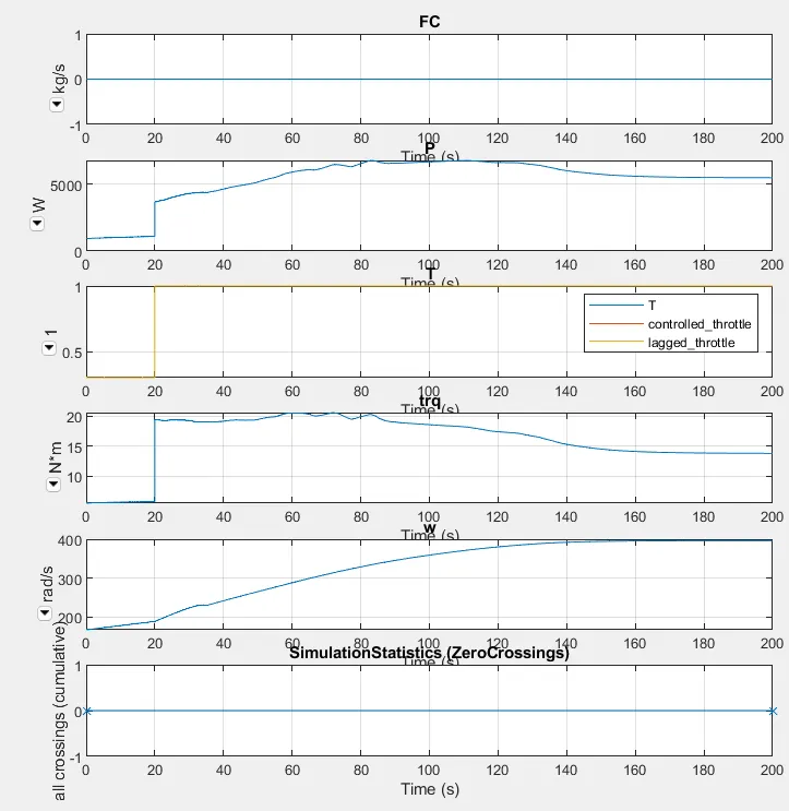
> Generic Engine:
> velocity,RPM,CVT Ratio plots: