Project

PROJECT REPORT

AIM: To carry out a system level simulation of an all-terrain vehicle.

OBJECTIVE: To download the model provided, run it and understand the system properties. The results should also be analysed.

MAJOR BLOCKS USED IN THE SYSTEM:

1. Generic Engine
2. Ideal Rotational Motion Sensor
3. Variable Ratio Transmission
4. Simple Gear
5. Double-Shoe Brake
6. Tire
7. Vehicle Body

MODEL ANALYSIS

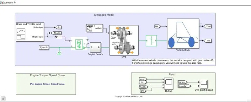
Here, a Generic Engine block is used for providing torque to the vehicle.

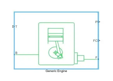
The block represents a system-level model of spark-ignition. The throttle input signal T takes the torque demanded from the engine as a fraction of the maximum possible torque as a physical signal. Connections F and B are mechanical rotational conserving ports associated with the engine crankshaft and engine block, respectively. Connections P and FC are physical signal output ports through which engine power and fuel consumption rate are reported, in this simulation these values are not taken into account.

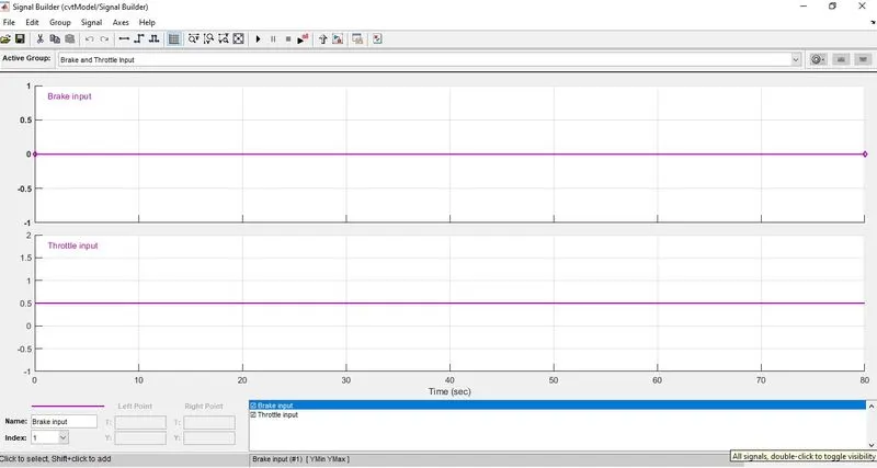
The torque requirement input value for the engine block is generated from a signal builder. The brake input values are also generated from this block.

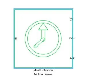
Then a subsystem senses the RPM output from the engine using a Ideal Rotational Motion Sensor. The RPM value is then plotted using a scope block.

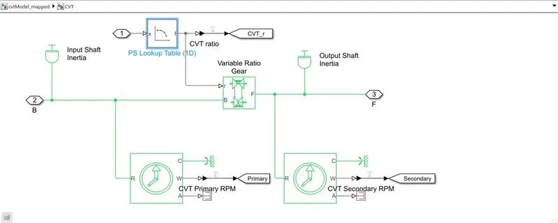
The Gearbox given here is a Continuously Variable Transmission (CVT) in a subsystem.

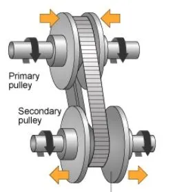
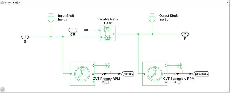
The main block of the subsystem is Variable Ratio Transmission Block which represents variable ratio gearbox such as implemented by mechanical belt CVT. Connections B (base) and F (follower) are mechanical rotational conserving ports.

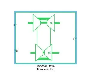
The physical signal input r defines the ratio of input to output angular shaft velocities which here is given as an input to the subsystem from a signal builder.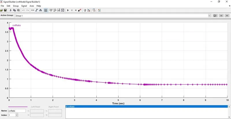

Inertia blocks are given before and after the transmission block to simulate the input and output shaft inertia given my the equations `m1*(((18.6e-2)/2)^2+((2.5e-2)/2)^2)/2` and `m2*(((19.8e-2)/2)^2+((1.9e-2)/2)^2)/2` where mi and m2 are declared in the workspace. Similarly Ideal Rotational Motion Sensor is also given before and after the variable transmission block to record the primary and secondary RPM in the shaft.

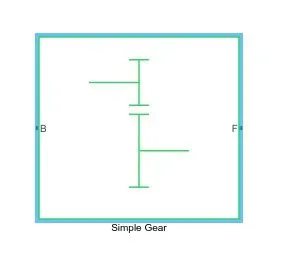
The next block in the system is a simple gear block, which represents a fixed-ratio gear or gear box. Connections B (base) and F (follower) are mechanical rotational conserving ports at a teeth ratio of 10 and the output shaft rotates in the same direction as the input shaft.

The engine power after the simple gear goes to the vehicle body subsystem which contains the brake system, four wheels and the vehicle body block.

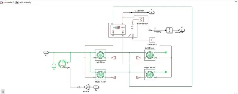
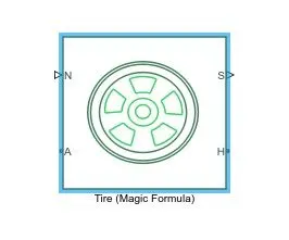
First the brake block is connected to the shaft, which is controlled by a physical signal made from the signal builder mentioned earlier. Then four Tire blocks are given to simulate the wheels of the ATV. These blocks represent the longitudinal behavior of a highway tire characterized by the tire Magic Formula. Connection A is the mechanical rotational conserving port for the wheel axle. Connection H is the mechanical translational conserving port for the wheel hub through which the thrust developed by the tire is applied to the vehicle. Connection N is a physical signal input port that applies the normal force acting on the tire. The force is considered positive if it acts downwards. Connection S is a physical signal output port that reports the tire slip.

The power from the axial is given to the rear wheels through the port A, making the ATV a rear wheel driven vehicle. The rear and front wheel forces are given by the vehicle body block which also calculates the velocity of the vehicle with respect to the thrust developed by the tires.

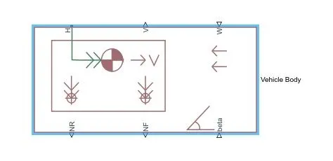
The vehicle body block represents a two-axle vehicle body in longitudinal motion. The block accounts for body mass, aerodynamic drag, road incline, and weight distribution between axles due to acceleration and road profile. Connection H is the mechanical translational conserving port associated with the horizontal motion of the vehicle body. The resulting traction motion developed by tires should be connected to this port. Connections V, NF, and NR are physical signal output ports for vehicle velocity and front and rear normal wheel forces, respectively. Wheel forces are considered positive if acting downwards. Connections W and beta are physical signal input ports corresponding to headwind speed and road inclination angle, respectively. In this case both the values are given as zero. The velocity value is then integrated to calculate the distance travelled.

Finally the throttle, brake, velocity and distance values are mapped in a scope given in a separate block set through goto blocks. The primary and secondary CVT shaft speeds are also plotted for reference. These plots show the results for this simulation model.

RESULTS

We are running the model for 200 seconds.

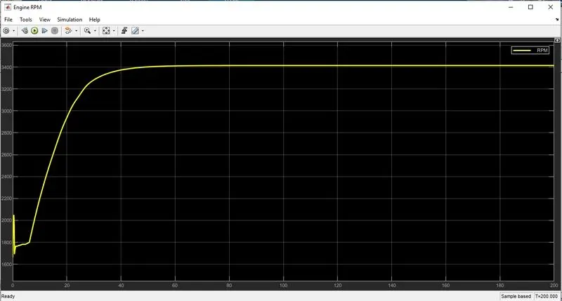
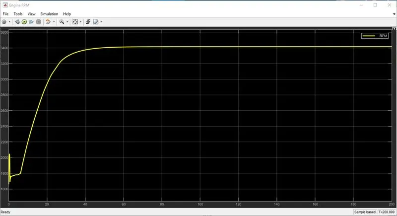
RPM of the generic engine is plotted against time as shown in the figure. We can observe that after some rise and dips in rpm value, it comes to a stable rate of 3400rpm after around 45 seconds.

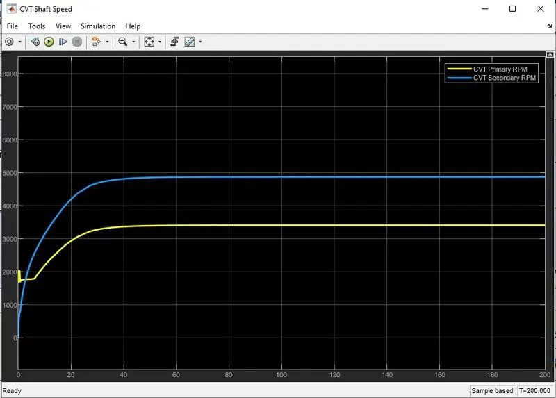
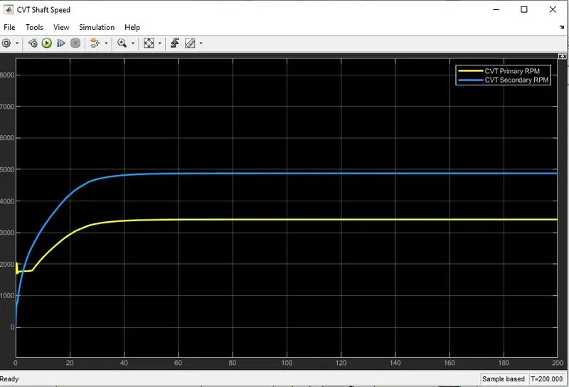
Here the change in rpm before and after the introduction of the gear system to the shaft can be observed. Secondary rpm gets higher than the primary rpm indicating a rise in the rpm value after the gear system in the axis.

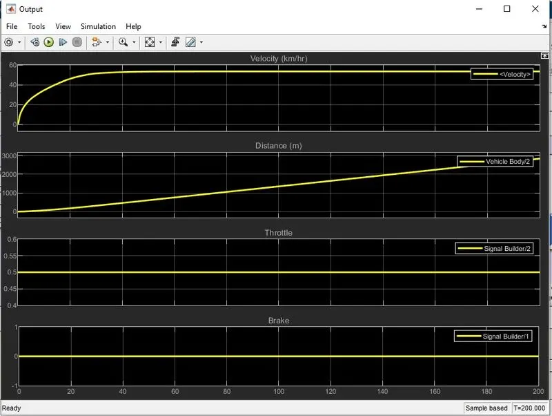
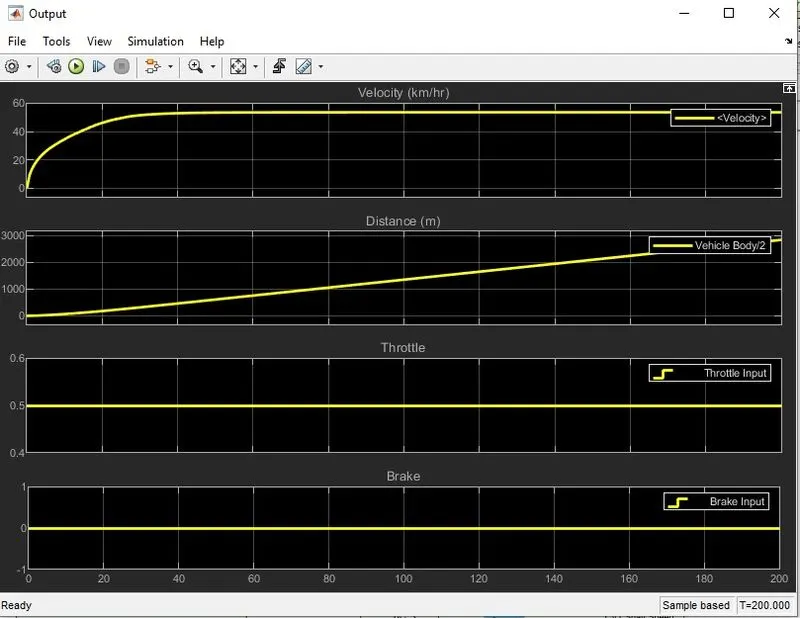
And finally the velocity, distance travelled, throttle input and brake input for the ATV can be seen here plotted against the simulation time. Velocity, like the engine rpm, reaches its maximum value of 53 km/hr right around after 45 seconds. ATV travelled a distance of 2830m in this time. The throttle input was a constant 0.5 throughout the simulation. Brake inputs were not given in this case.

2. ATV Model with Dashboard.

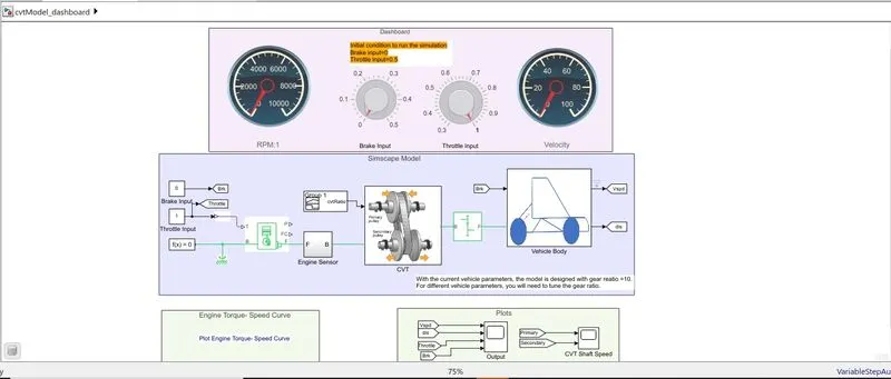
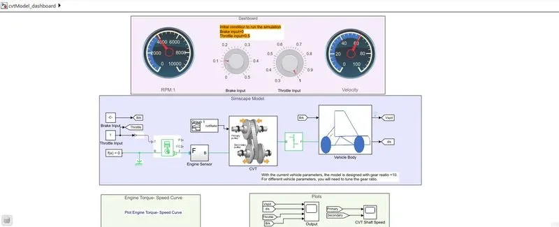
This model has a dashboard where the inputs of throttle and brake can be given by the user during the simulation. This is achieved using two knob blocks connected to two separate constant blocks which then passes the respective values to throttle and brake inputs. The dashboard also contains two circular gauge blocks which show the RPM of the engine and velocity of the vehicle in real time. This feature makes the model more user friendly and studies on different inputs of the user’s choice can be achieved. All the other aspects of the model are the same as the previous one.

RESULTS

The initial condition to run the simulation is given as brake input = 0 and throttle input = 0.5.

The engine RPM is the same as the previous case as the throttle input is the same. Reaching the maximum value of 3400 rpm around 45 seconds.

No significant changes in the primary and secondary RPMs of the gear system compared to the earlier case.

Values of velocity, distance travelled, throttle input and brake inputs are also similar to the previous case.

SIMULATION RUN 2 of ATV Model with Dashboard.

Now the same model is run with different inputs. The throttle input is raised to 1 and brake input to 0.1.

RESULTS

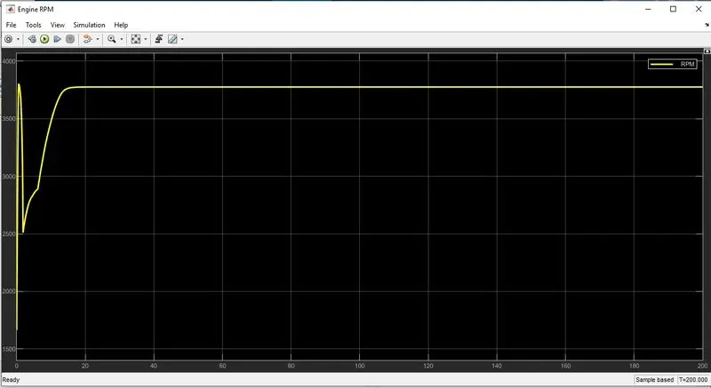
The increase in throttle input is reflected in the engine RPM as it reaches a maximum value of 3778 in 20 seconds.

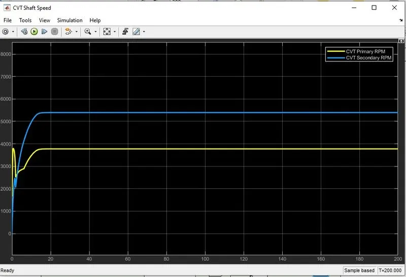
Even though the values of primary and secondary RPMs have increased as the engine rpm, it’s characteristics remain the same.

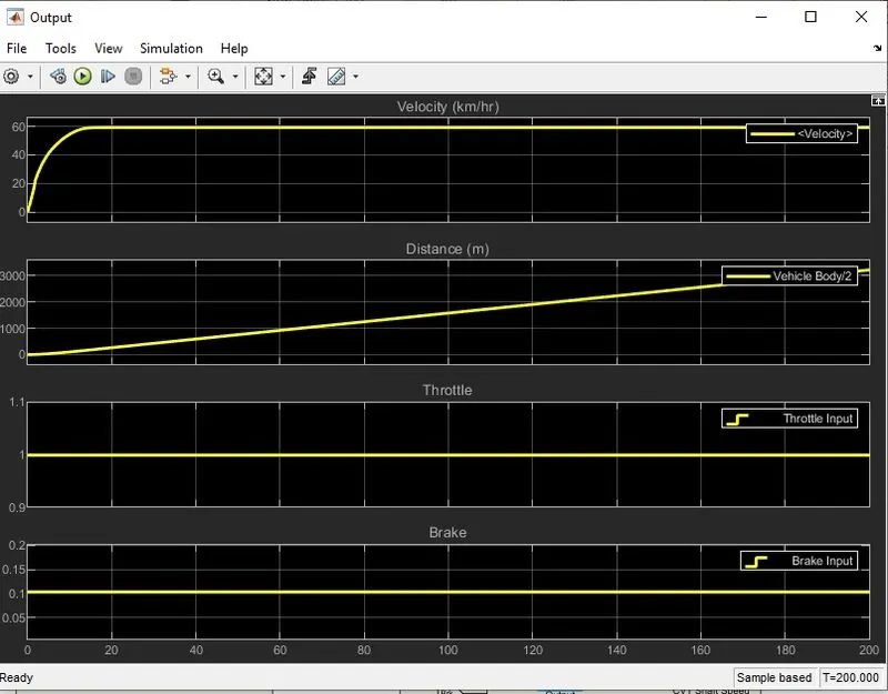
Similar increases in the velocity and distance travelled can also be observed. This time the vehicle archives a maximum velocity of 59.19 km/hr after 30 seconds and the distance travelled is 3215m. The given inputs of throttle and brake are also visible in the figure.

3. ATV MODEL with PSLookup Table

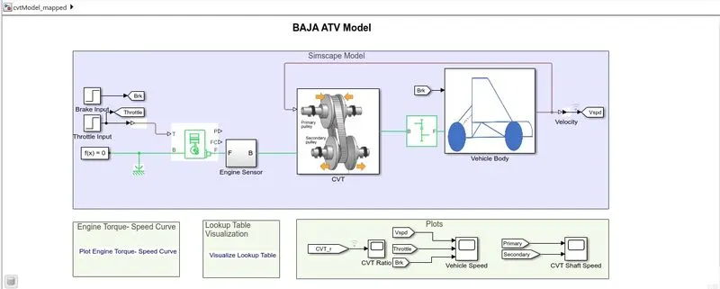
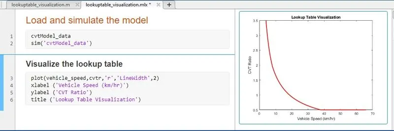
This model differs from the first model in two aspects. The inputs for throttle and brake are given using two separate Step blocks and the gear ratios are given from a datatable using PS Lookup table. This table gives the physical signal input r, which is the ratio of input to output angular shaft velocities, to the Variable Ratio transmission. PS Lookup table represents a physical signal converter whose input-output relationship is specified by a lookup table. The table gives the ratio value with respect to the values of velocity. All the other blocks and connections are same as the first model.

The PS Lookup table connected to the variable ratio gear can be observed here. The table takes the velocity value as input and gives the corresponding gear ratio to the system.

Lookup Table Visualization

RESULTS

The results for this model are analysed below.

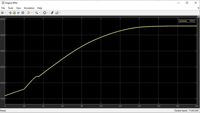
Since the throttle input is generated from a step block the engine RPM rises more gradually over the time period reaching maximum RPM of 3780 after 150 seconds.

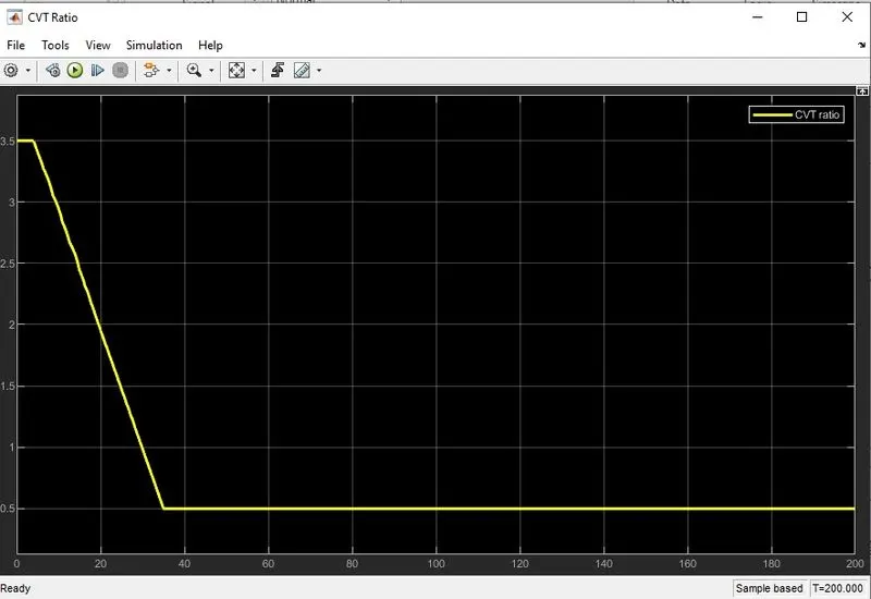
The gear ratio produced from the lookup table is plotted against time here. It starts from 3.5, then drops to 0.5 in 30 seconds and maintains the value throughout.

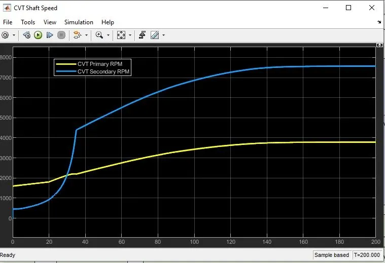
The change in gear ratio given from the lookup table is visible in the secondary RPM values as it behaves differently from the primary RPM value and it reaches a higher RPM value compared to previous cases.

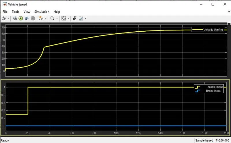
Similarly the change in velocity can also be observed. It follows a certain curve till 34 seconds and a less gradient slope after that. ATV achieves its highest velocity of 65 km/hr after 140 seconds.

4. Dashboard attached to ATV MODEL with PSLookup Table

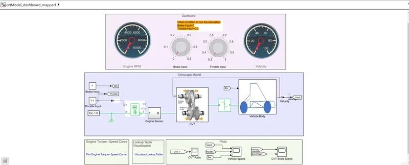
This model has a dashboard where the inputs of throttle and brake can be given by the user during the simulation. This is achieved using two knob blocks connected to two separate constant blocks which then passes the respective values to throttle and brake inputs. The dashboard also contains two circular gauge blocks which show the RPM of the engine and velocity of the vehicle in real time. This feature makes the model more user friendly and studies on different inputs of the user’s choice can be achieved. All the other aspects of the model are the same as the previous one.

RESULTS

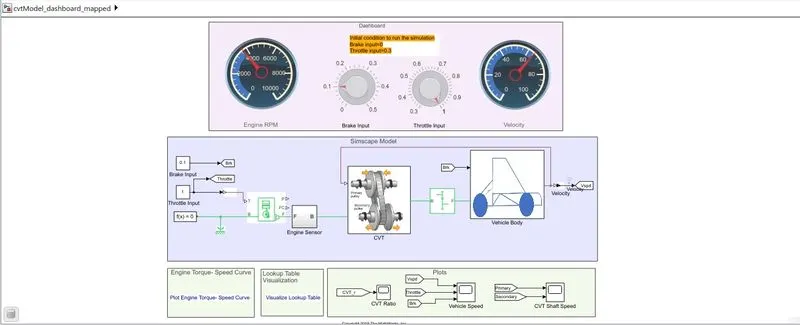
The initial condition to run the simulation is given as brake input = 0 and throttle input = 0.3

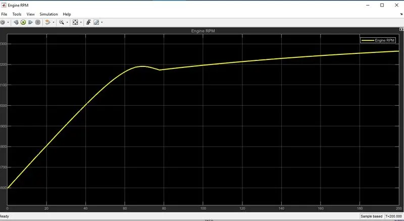
The engine RPM increases steadily for 68 seconds reaching 2190rpm and then takes a slight dip, then continues rising with a lesser slope throughout the simulation, reaching a value of 2260 RPM at the end.

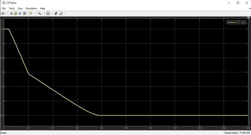
The gear ratio produced from the lookup table is plotted against time here. It starts from 3.5, then drops to 1.93 in 17 seconds and continues the drop with a different slope till 77 seconds coming down to a value of 0.5.

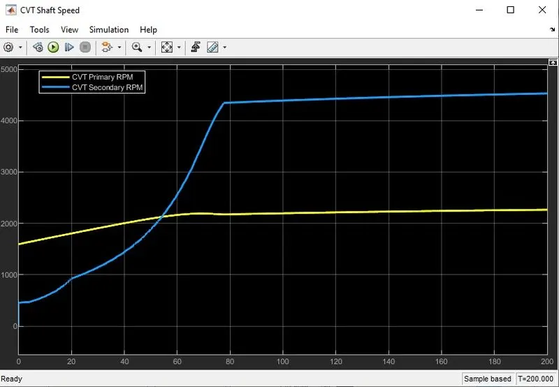
The change in gear ratio given from the lookup table is visible in the secondary RPM values as it behaves differently from the primary RPM value and it reaches a higher RPM value compared to previous cases.

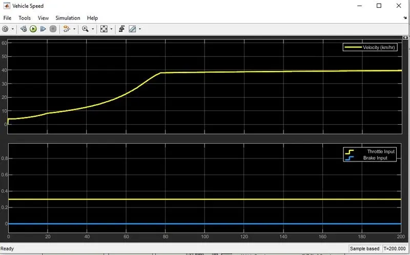
Velocity of the ATV increases significantly for 80 seconds reaching 78 km/hr and then maintains the velocity throughout. The throttle and brake inputs can also be observed in the figure.

SIMULATION RUN 2 of Dashboard attached to ATV MODEL with PSLookup Table.

Now the same model is run with different inputs. The throttle input is raised to 1 and brake input to 0.1.

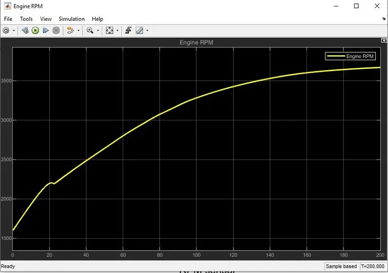
A gradual increase in the engine RPM can be observed here. The value keeps on increasing throughout the simulation reaching a maximum value of 3670rpm.

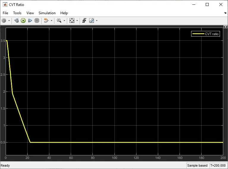
The structure of the CVT ratio graph is similar to that of the previous case but here the drop happens more suddenly, starting from 3.5 then dropping to 1.93 in 6 seconds and continues the drop with a different slope till 22 seconds coming down to a value of 0.5.

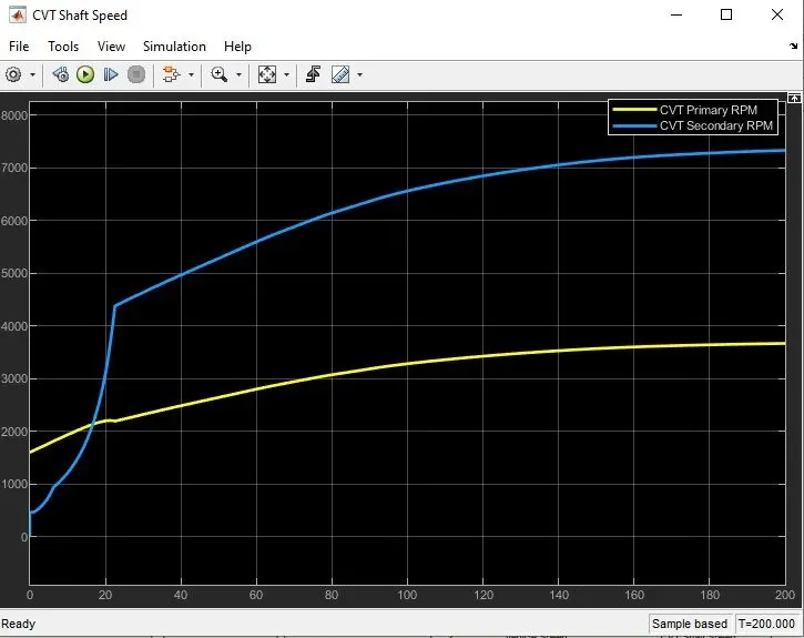
As mentioned in case of CVT ratio, here also we can observe the same graph structure as the previous case but happening more suddenly.

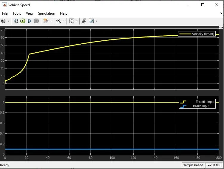
Finally the velocity of the ATV can be observed here where it increases rapidly for 22 seconds reaching 38 km/hr and then a more less slope increase throughout the simulation reaching 63 km/hr at the end. The throttle and brake inputs can also be observed in the figure.

CONCLUSION

The four models of the ATV are analysed successfully and the properties of these models are discussed in the report.