Project

Aim: A case study of system-level simulation of a BAJA all-terrain vehicle.

Objectives: To Prepare a technical report explaining the model properties & comments on the results.

All Terrain Vehicle:(ATV)

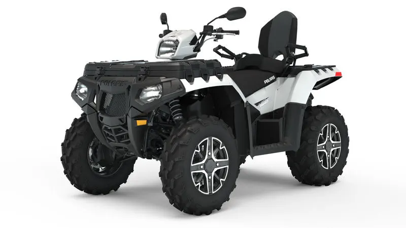
Figure 2: ATV

An all-terrain vehicle (ATV) is defined as a motorized off-highway vehicle designed to travel on four low-pressure or non-pneumatic tires, having a seat designed to be straddled by the operator and handlebars for steering control. ATVs are subdivided into two types as designated by the manufacturer. Type I ATVs are intended by the manufacturer for use by a single operator and no passenger. Type II ATVs are intended by the manufacturer for use by an operator and a passenger, and are equipped with a designated seating position behind the operator.

Continuously Variable Transmission: (CVT)

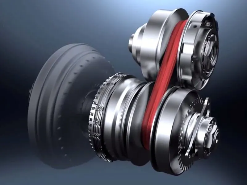
Figure 1: CVT

A Continuously Variable transmission (CVT) is an automatic transmission that can change seamlessly through a continuous range of gear ratios. This contrasts with other transmissions that provide a limited number of gear ratios in fixed steps. The flexibility of a CVT with suitable control may allow the engine to operate at a constant RPM while the vehicle moves at varying speeds.

In order to increase the output obtained from the engine without modifying the engine, a Continuously Variable Transmission (CVT) must be used. A CVT transmits power from the engine to the wheels by changing the diameter of the CVT cones. It can also adjust a vehicle’s engine’s torque in an infinite number of ways. This makes a CVT far more efficient than a normal gearbox. By properly tuning the CVT, it is possible to improve the vehicle’s power output while ensuring that the vehicle is still fuel efficient. Additionally, since a CVT functions similarly to an automatic transmission, no pneumatic clutch is required in this system since it is powered by a torque converter. CVT’s are desirable in this situation because they have a large range of transmission ratios, are lightweight and easy to tune.

Common Model Blocks:

Generic Engine:

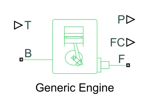
The Generic Engine block represents a general internal combustion engine. Engine types include spark-ignition and diesel. Speed-power and speed-torque parameterizations are provided. A throttle physical signal input specifies the normalized engine torque. Optional dynamic parameters include crankshaft inertia and response time lag. A physical signal port outputs engine fuel consumption rate based on choice of fuel consumption model. Optional speed and redline controllers prevent engine stall and enable cruise control.

The throttle input signal T lies between zero and one and specifies the torque demanded from the engine as a fraction of the maximum possible torque. If the engine speed falls below the Stall speed, the engine torque is blended to zero. If the engine speed exceeds the Maximum speed, the simulation stops and issues an error message.Connections F and B are mechanical rotational conserving ports associated with the engine crankshaft and engine block, respectively. Connections P and FC are physical signal output ports through which engine power and fuel consumption rate are reported.

Variable Ratio Transmission:

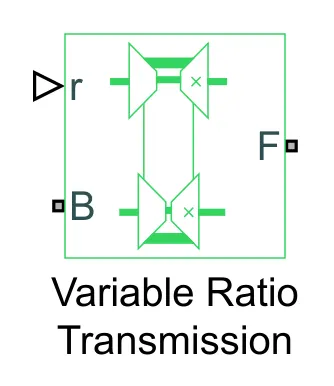
The Variable Ratio Transmission block represents a gearbox that dynamically transfers motion and torque between the two connected drive shaft axes, base and follower. A variable ratio gearbox such as implemented by mechanical belt CVT, electric, or hydraulic transmissions. The physical signal input r defines the ratio of input to output angular shaft velocities. Connections B (base) and F (follower) are mechanical rotational conserving ports. Specify the relation between base and follower rotation directions with the Output shaft rotates parameter.

Simple Gear:

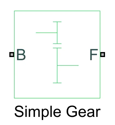
The Simple Gear block represents a gearbox that constrains the connected driveline axes of the base gear, B, and the follower gear, F, to corotate with a fixed ratio that you specify. You choose whether the follower axis rotates in the same or opposite direction as the base axis. If they rotate in the same direction, the angular velocity of the follower, ωF, and the angular velocity of the base, ωB, have the same sign. If they rotate in opposite directions, ωF and ωB have opposite signs.

Vehicle Body:

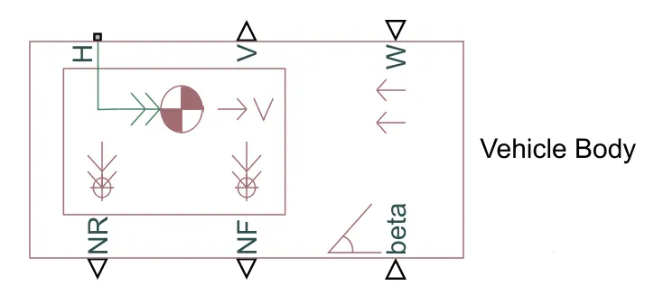
The Vehicle Body block represents a two-axle vehicle body in longitudinal motion. The vehicle can have the same or a different number of wheels on each axle. The vehicle wheels are assumed identical in size. The vehicle can also have a center of gravity (CG) that is at or below the plane of travel. The block accounts for body mass, aerodynamic drag, road incline, and weight distribution between axles due to acceleration and road profile. Optionally include pitch and suspension dynamics. The vehicle does not move vertically relative to the ground. The block has an option to include an externally-defined mass and an externally-defined inertia. The mass, inertia, and center of gravity of the vehicle body can vary over the course of simulation in response to system changes.

Case 1: Study the BAJA ATV model.

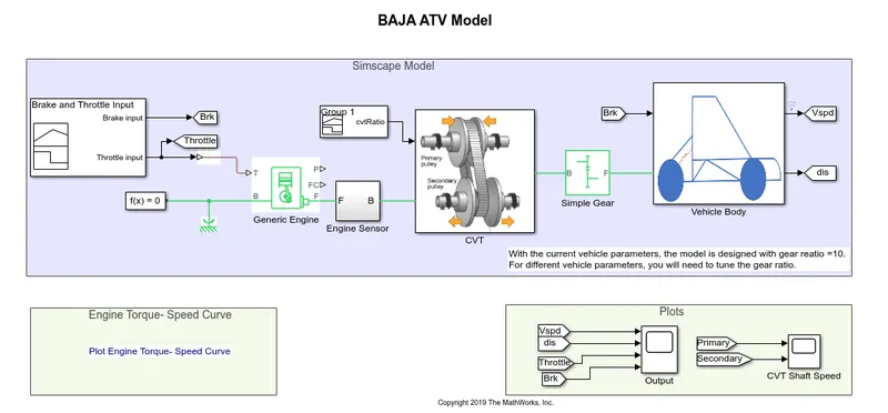
Figure 3: ATV Model

• In the above figure the BAJA ATV model shows. For this model several blocks are used.
• For brake and throttle signal builder are used in this signal builder, brake signal is 0 and throttle signal is 0.5.
• In the engine block speed and torque parameter fetch from Engine speed torque curve, it shows in below fig. 4 also selected interpolation method is linear. Engine sensor is nothing but an ideal rotational motion sensor block its determine engine RPM.

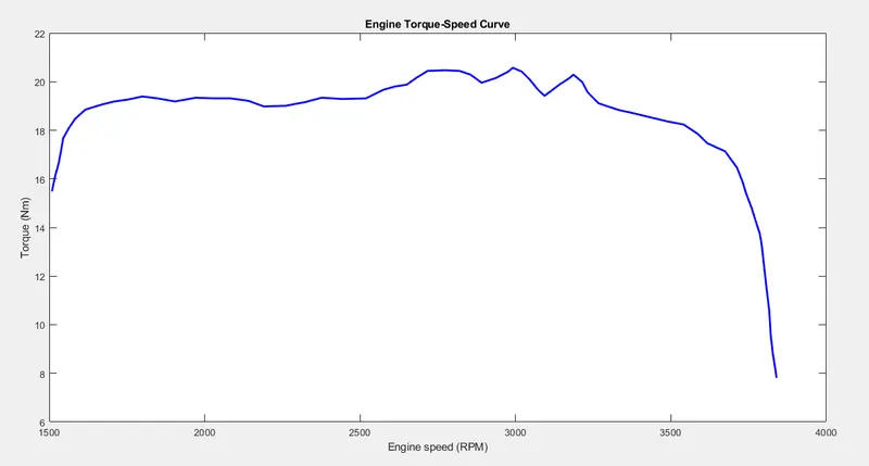
Figure 4: Engine Torque-Speed Curve

• Below fig. 5 shows the inside model of continuous variable transmission (CVT). This used inertia, ideal rotational motion sensor, variable ratio transmission, etc.

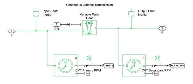
Figure 5 CVT Model

• Required cvt ratio signal for variable ratio gear, build in signal builder and its look like below fig. 6.
• Also in CVT used inertia block for input shaft inertia and output shaft inertia and its value are 3.5 kg*m^2 and 3.2 Kg*m^2.

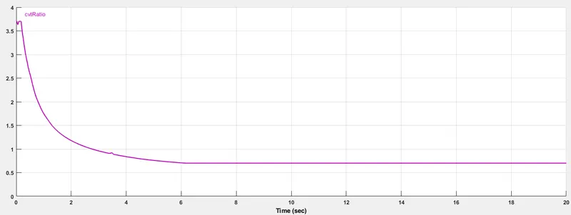
Figure 6: CVT Ratio Signal

• Simple Gear is a physical simscape block, its work as fixed or variable gearbox and its teeth ratio is 10.
• Below fig. 7 shoes inside the model of vehicle body, this used vehicle body, tier, double shoe brake, etc.

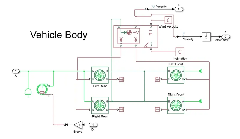
Figure 7: Vehicle Body Model

• The vehicle body model determines velocity of vehicle and displacement travelled by vehicle.
• Below fig. 8 shows graph of output result velocity, displacement, and input brake, throttle signal
• Similarly, fig. 9 shows primary and secondary CVT shaft speed curve.

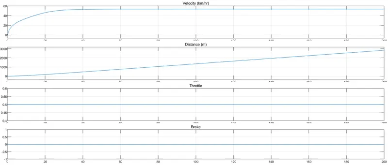
Figure 8

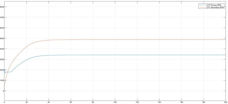
Figure 9

Case 2: Study the BAJA ATV model with Dashboard.

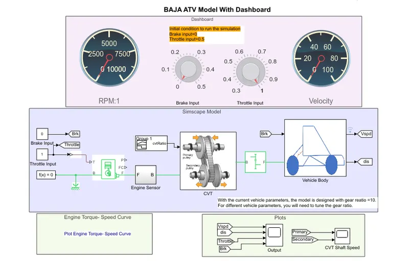
Figure 10: ATV Model with Dashboard

• Above fig. 10 shows an ATV Model with dashboard. It is similar to case 1 model only difference is, now brake and throttle input controlled by the user.
• Below fig. 11 and 12 shows graphs of scope output and CVT Shaft Speed respectively.

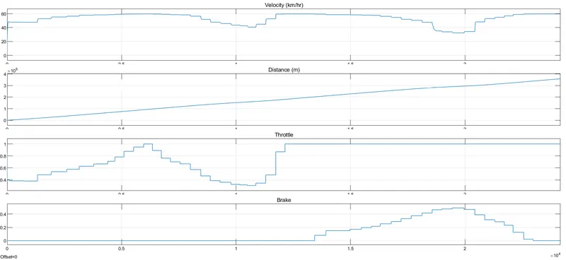
Figure 11

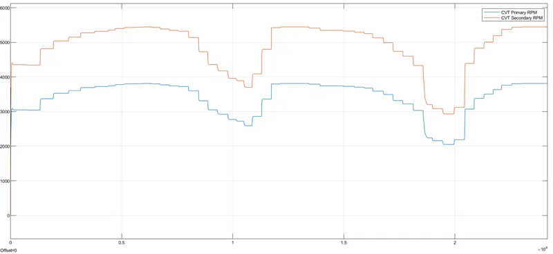
Figure 12

Case 3: Study the BAJA ATV model using a Lookup table.

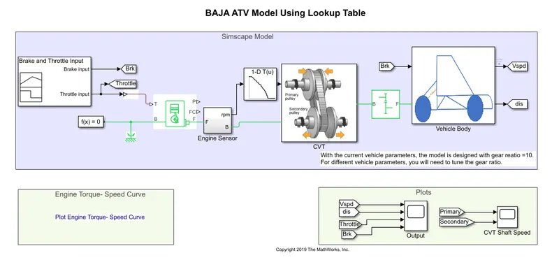
Figure 13: ATV Model by using Lookup Table

• In above fig. 13 shows the ATV Model by using a lookup table. It is similar to case 1 model except the lookup table.
• Instead of the cvt ratio graph used the 1-D lookup table and calculate the cvt ratio by using cvtr (i.e. below fig. 14 graph) as a tabledata, speedV (i.e. speed value of engine speed torque curve shown in fig. 4) as a breakpoint1 data and engine RPM gave an input signal.

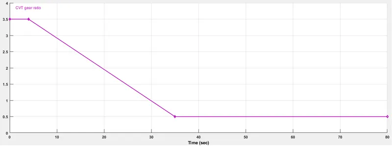
Figure 14: cvtr graph

• Below fig. 15 and 16 shows graphs of scope output and CVT Shaft Speed respectively.

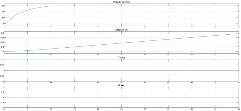
Figure 15

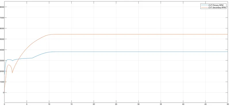
Figure 16

Case 4: Study the BAJA ATV model using a Lookup table with Dashboard.

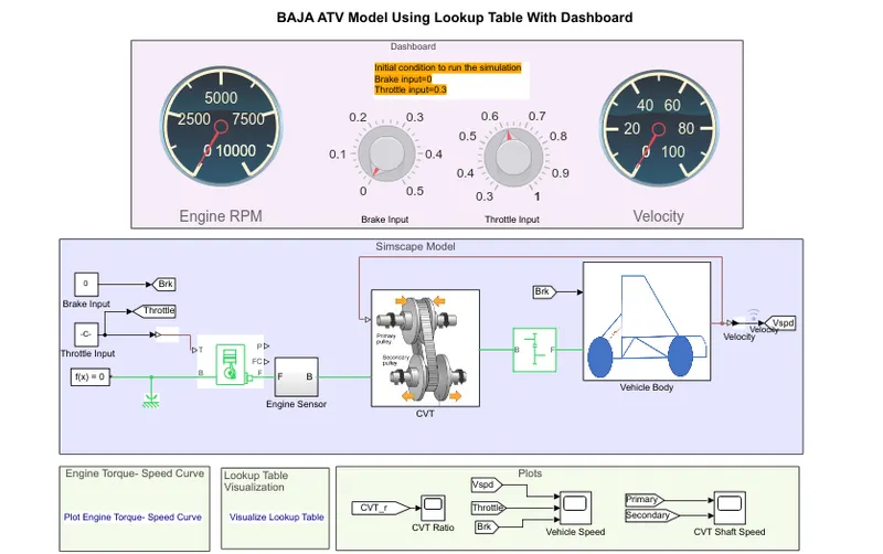
Figure 17: ATV Model using Lookup Table with Dashboard

• In above fig. 17 shows the ATV Model by using a lookup table with dashboard. It is similar to case 2 model except the lookup table.
• The lookup table is similar close to case 3 lookup table, just different is, now they used input signal as vehicle velocity instead of engine RPM.
• Below fig. 18 shows the lookup table visualization.

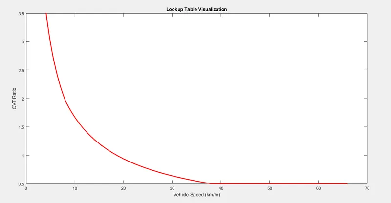
Figure 18: Lookup Table Visualization

• As per the fig. 18 when vehicle speed increases CVT ratio decreases.
• Below fig. 19 and 20 shows graphs of scope output and CVT Shaft Speed respectively.

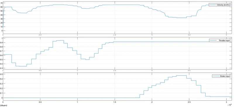
Figure 19

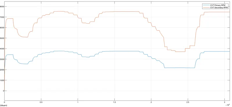
Figure 20

Conclusion:

• When the throttle is increased or break is decreased, the speed of the vehicle increases and vice versa.
• Fluctuation in CVT shaft speed is more when the lookup table was used as compared to without lookup table model.