Project
Objective: To study the BAJA ATV model that was built using MATLAB Simulink and prepare technical report on it.
Description:
BAJA:
Baja SAE is a Collegiate Design Series competition run by the Society of Automotive Engineers International (SAE International). Teams of students from universities all over the world design and build small off-road cars. The cars all have engines of the same specifications. The goal in Baja SAE racing is to design, build and race off-road vehicles that can withstand the harshest elements of rough terrain. The vehicles used in Baja SAE racing are often similar in appearance to dune buggies.
All-Terrain Vehicle:
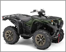
Yamaha ATV
An all-terrain vehicle (ATV), also known as a light utility vehicle (LUV), a quad bike, or simply a quad, as defined by the American National Standards Institute (ANSI), is a vehicle that travels on low-pressure tires, with a seat that is straddled by the operator, along with handlebars for steering control. As the name implies, it is designed to handle a wider variety of terrain than most other vehicles. India saw the launch of the event (BAJA SAE) in January 2007. Since last five years, Mahindra has been the title sponsor for the event.
The rider sits on and operates these vehicles like a motorcycle, but the extra wheels give more stability at slower speeds. Although most are equipped with three or four wheels, six-wheel models exist for specialized applications. Multiple-user analogues with side-by-side seating are called utility terrain vehicles (UTVs) or side-by-sides to distinguish the classes of vehicle. Both classes tend to have similar powertrain parts.
Continuous variable transmission (CVT):
It is a new technology used in automobiles which provides more gear ratios and makes the automobile movement smooth. The basic components of the CVT are, two pulleys, steel belt and sometimes planetary gear set is used if reverse gear is required.
There are two conditions that are obtained from CVT,
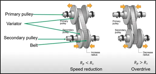
a. Speed reduction:
When the variators of the primary pulley move aside by increasing gap between them the effective diameter of the primary pully decreases. Simultaneously, the variators of secondary pulley are moved towards each other by decreasing the gap which increases the effective diameter of secondary pulley and this causes the speed reduction of the vehicle.
b. Overdrive:
When the variators of the Secondary pulley move aside by increasing gap between them the effective diameter of the secondary pully decreases. Simultaneously, the variators of primary pulley are moved towards each other by decreasing the gap which increases the effective diameter of secondary pulley and this is causes increased speed termed as overdrive.
The major Simscape block used in BAJA ATV models.
Generic engine:
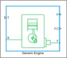
It is a Simscape block representing a system-level model of spark-ignition and diesel engines suitable for use at initial stages of modelling when only the basic parameters are available. Speed-power and speed-torque parameterizations are provided. A throttle physical signal input specifies the normalized engine torque. Optional dynamic parameters include crankshaft inertia and response time lag. A physical signal port outputs engine fuel consumption rate based on choice of fuel consumption model. Optional speed and redline controllers prevent engine stall and enable cruise control.
By default, the Generic Engine model uses a programmed relationship between torque and speed, modulated by the throttle signal.
Ports:
- B -Rotational conserving port representing the engine block.
- F - Rotational Conserving port representing the engine crankshaft.
- T - Physical signal input port specifying the normalized engine throttle level.
- P - Physical signal output port reporting the instantaneous engine power, in W.
- FC - Physical signal output port reporting the fuel consumption rate, in kg/s.
Ideal rotational motion sensor:
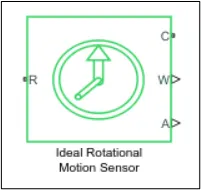
The block represents an ideal mechanical rotational motion sensor, that is, a device that converts an across variable measured between two mechanical rotational nodes into a control signal proportional to angular velocity or angle. The sensor is ideal since it does not account for inertia, friction, delays, energy consumption, and so on.
Connections R and C are mechanical rotational conserving ports and connections W and A are physical signal output ports for velocity and angular displacement, respectively.
Ports:
- R - Mechanical rotational conserving port associated with the sensor positive probe.
- C - Mechanical rotational conserving port associated with the sensor negative (reference) probe.
- W - Physical signal output port for angular velocity.
- A - Physical signal output port for angular displacement.
Variable ratio transmission:
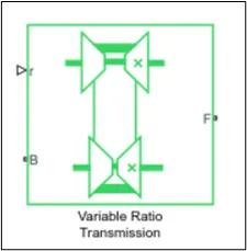
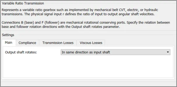
It is a Simscape block representing a gearbox that dynamically transfers motion and torque between the two connected driveshaft axes, base and follower. Ignoring the dynamics of transmission compliance, the driveshafts are constrained to corotate with a variable gear ratio that you control. You can choose whether the follower axis rotates in the same or opposite direction as the base axis. If they rotate in the same direction, ωF and ωB have the same sign. If they rotate in opposite directions, ωF and ωB have opposite signs.
Ports:
- r - Physical input signal.
- B - Base driveshaft.
- F – Follower driveshaft.
Simple gear:
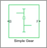
It is a Simscape block representing a fixed ratio gear. No inertia or compliance is modelled in this block. Options to whether to include gear meshing and viscous bearing losses or not is up to the users designed model. Other data such as Meshing losses, Viscous losses can be added. Optionally include thermal effects and expose thermal conserving port H by right-clicking on the block and selecting Simscape block choices to switch between variants.
Ports:
- B - Mechanical rotational conserving port (Input).
- F - Mechanical rotational conserving port (Output).
Vehicle body:
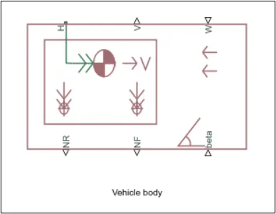
It is a Simscape block representing a two-axle vehicle body in longitudinal motion. The vehicle can have the same or a different number of wheels on each axle. For example, two wheels on the front axle and one wheel on the rear axle. The vehicle wheels are assumed identical in size. The vehicle can also have a centre of gravity (CG) that is at or below the plane of travel.
The block accounts for body mass, aerodynamic drag, road incline, and weight distribution between axles due to acceleration and road profile. Optionally include pitch and suspension dynamics. The vehicle does not move vertically relative to the ground. The block has an option to include an externally-defined mass and an externally-defined inertia. The mass, inertia, and centre of gravity of the vehicle body can vary over the course of simulation in response to system changes.
Ports:
- W - Physical signal input port for headwind speed.
- Beta - Physical signal input port for road incline angle.
- H - Conserving port associated with the horizontal motion of the vehicle body. Connect tire traction motion to this port.
- NR - Physical signal output port for normal force on the rear axle. Wheel forces are considered positive if acting downwards.
- NF - Physical signal output port for normal force on the front axle. Wheel forces are considered positive if acting downwards.
- V - Physical signal output port for vehicle longitudinal velocity.
Tire:
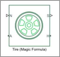
It is a Simscape block representing a tire with longitudinal behaviour given by the Magic Formula, an empirical equation based on four fitting coefficients. The block can model tire dynamics under constant or variable pavement conditions. The longitudinal direction of the tire is the same as its direction of motion as it rolls on pavement.
To increase the fidelity of the tire model, you can specify properties such as tire compliance, inertia, and rolling resistance. However, these properties increase the complexity of the tire model and can slow down simulation. Consider ignoring tire compliance and inertia if simulating the model in real time or if preparing the model for hardware-in-the-loop (HIL) simulation.
Ports:
- N - Physical signal input port associated with the normal force acting on the tire. The normal force is positive if it acts downward on the tire, pressing it against the pavement.
- A - Mechanical rotational port associated with the axle that the tire sits on.
- H - Mechanical translational port associated with the wheel hub that transmits the thrust generated by the tire to the remainder of the vehicle.
- S - Physical signal output port associated with the relative slip between the tire and road.
Double Shoe Brake:
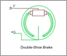
It is a Simscape block that represents the Double-Shoe Brake block represents a frictional brake with two pivoted rigid shoes that press against a rotating drum to produce a braking action. The rigid shoes sit inside or outside the rotating drum in a diametrically opposed configuration. A positive actuating force causes the rigid shoes to press against the rotating drum. Viscous and contact friction between the drum and the rigid shoe surfaces cause the rotating drum to decelerate.
Double-shoe brakes provide high braking torque with small actuator deflections in applications that include motor vehicles and some heavy machinery. The model employs a simple parameterization with readily accessible brake geometry and friction parameters.
Ports:
- F - Physical signal input port associated with the applied actuating force.
- S - Rotational conserving port associated with the rotating drum shaft.
1. BAJA ATV Model
Simulink model of BAJA ATV model:
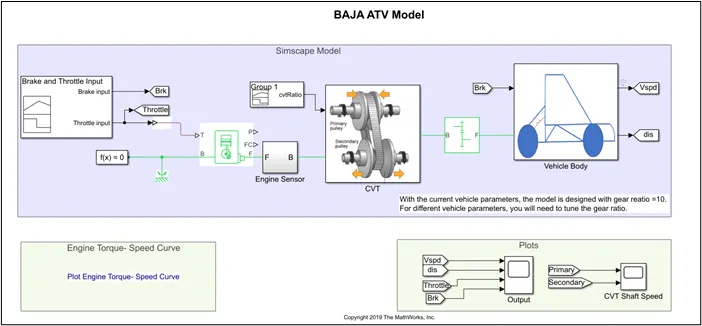
Form the above ATV model, the input is provided through the signal builder consisting of two separate signals namely, Throttle and Brake input. Where, Throttle of 0.5 and Brake value 0 is provided constantly as shown in below figure. These two signals are tagged using ‘Goto’ tag, so that they can be used as input for other blocks/sub-systems.
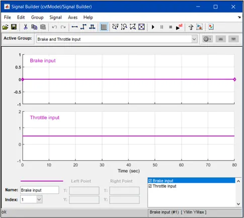
Signal builder dialog box.
The throttle signal is provided to the Generic engine block as input through ‘Simulink-PS converter’ (converts Simulink signal to physical signal). Following are the parameters that are defined for the generic engine block
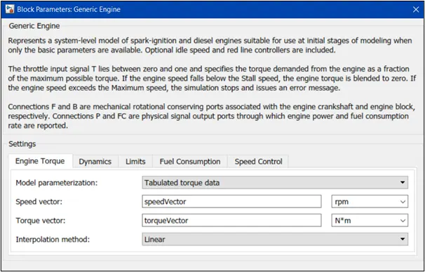
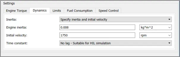
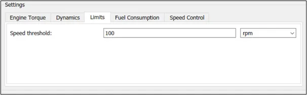
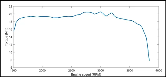
The torque and speed vector for the generic engine block is extracted from the below image using one of the file exchanges ‘GRABIT ‘. Through which all the data points from the image are extracted and fed as input to the blocks.
Engine subsystem block:
Engine sensor is one of the sub systems of the model through which the output signal of the Generic engine is connected to the CVT. This sub system consists of an Ideal rotational motion sensor to record the RPM of the generic engine. The signal (signal of the Generic engine connecting to the CVT.) passes through the port R, C is connected to Mechanical rotational reference, W gives the variations that are occurred when the model is turned ON and this is connected to a scope to observe the output graphically.
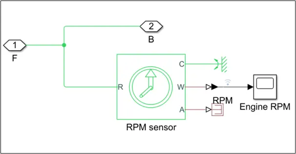
Engine sensor sub system.
CVT subsystem block:
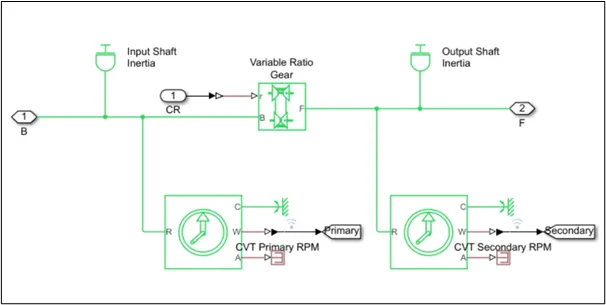
CVT sub system.
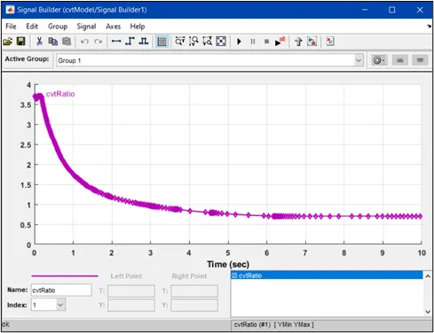
Signal builder for CVT ratio.
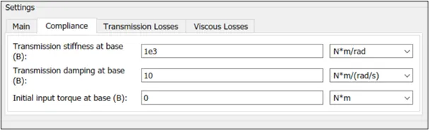
The signal passing through the engine sensor is connected to the port B of the Variable ratio transmission (named as Variable ratio gear for this model) and the CVT ratio (built using signal builder) is connected to port r. The output of the Variable ratio gear (secondary shaft) is connected to a simple gear block in the Simulink canvas. Two rotational motion sensors are used for both the shafts (Primary and Secondary) to record the RPM and the output from both are tagged using the ‘Goto’ tag and are connected to a scope outside the CVT sub system. The below snaps show the parameters that are defined for the Variable ratio transmission block.
Vehicle body subsystem block:
The CVT and Vehicle body sub stations are connected through a simple gear block with a constant gear ratio of 10.
The vehicle sub system consists Vehicle body block, tire blocks, Double-shoe brake and few other Simscape blocks which are connected as shown in below snap.
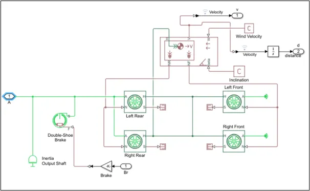
Vehicle body sub system.
The below image shows the parameters defined for the vehicle body block,
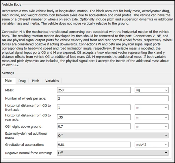
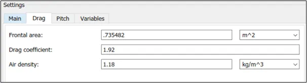
- The shoe brake is connected to rear tires and the front tires are left free by connecting the port A to Rotational free end block. The brake that was tagged is now connected to the Shoe brake block as input through a gain block (gain of 1000).
- From port V of the vehicle body block the velocity and the displacement (by passing the signal through the Integrator block) can be observed graphically, both Velocity and Distance are tagged and connected to a scope outside the sub system.
Output:
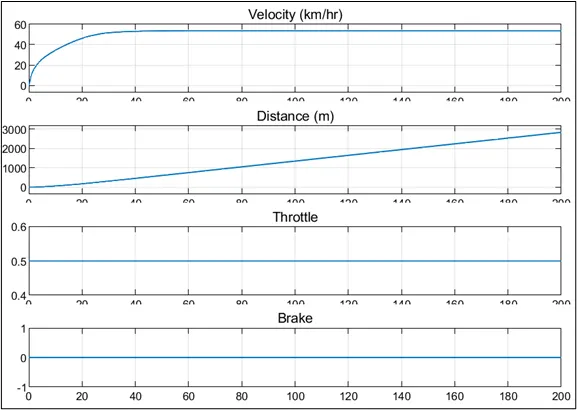
From the above snap it can be seen that for Throttle o.5 and brake value of 0, velocity increases for first 40 seconds and then it remains constant at around 53km/hr. The Distance moved by the vehicle also increases gradually.
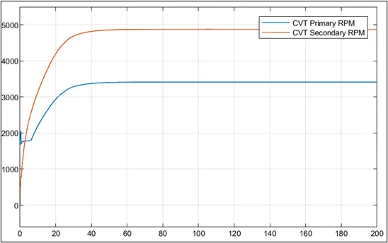
The above graph shows
- The rpm of primary shaft of CVT (input shaft of Variable ratio transmission) increases from 0 to 40 second (with some variations) around 3300rpm and remains constant till end (200 sec).
- The rpm of secondary shaft (output shaft of Variable ratio transmission) increases from 0 to 40 second to 4800rpm and then remains constant till end, which is less compared to the primary shaft. The graphical nature of RPM of CVT secondary shaft is similar to the speed of the vehicle.
*For the same model with the Throttle, Brake and CVT ratio values as shown in below figure the following output was obtained.*
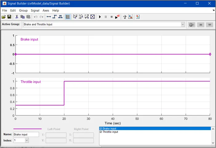
Signal builder for Brake and Throttle input to the model.
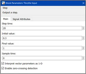
In the above image it can be observed that the barke is maintained zero till last and the throttle value from 0 to 20 seconds was maintained 0.3 and then from 20seconds till last it was kept constant at 1.
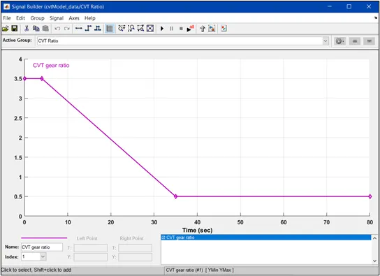
CVT ratio along time.
The ratio for first few seconds was constant (3.5) and for time period 3 to 35 seconds was reduced to 0.5 and further it was kept constant and this ratio was fed to the CVT subsystem of the above ATV model.
Output for above shown Throttle, Brake & CVT ratio values:
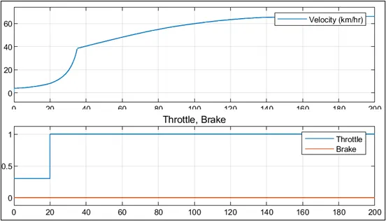
In the graph we can observe the velocity got increased to 65km/hr with max throttle value.
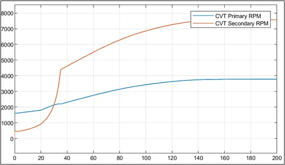
The RPM of primary shaft was increasing gradually to 3800rpm and the rpm of secondary shaft was more (7500rpm) compared to primary CVT shaft. The graphical nature of RPM of CVT secondary shaft is similar to the speed of the vehicle.
2. BAJA ATV Model with dashboard:
Simulink model for BAJA ATV model with dashboard:
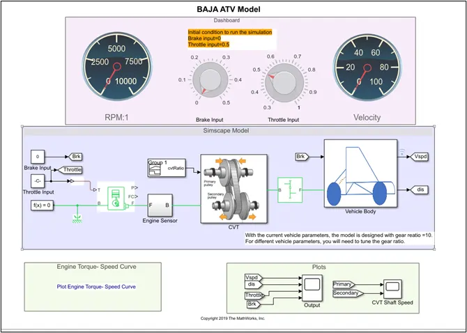
The above is the BAJA ATV model with dashboard, everything in this model is same as BAJA ATV model (without dashboard) except the dashboard and the input fed to the generic engine.
The dashboard consists of two Custom gauges (one for indicating the RPM at the engine sensor another for indicating the velocity of the vehicle body block) and two Knobs (one as Brake input another Throttle input).
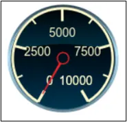
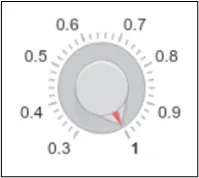
Custom gauge Knob
For both dashboard components minimum and maximum limit with the tick interval need to be provided.
Using the knobs, we can alter the brake and throttle values as per the requirement and the results can be observed respectively.
Output:
The knob of Throttle and Brake were varied randomly during simulation and following results were obtained.
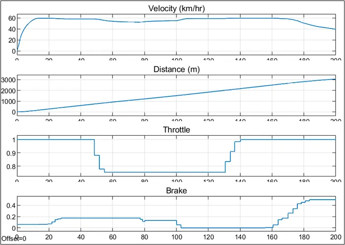
From the above graph it can be observed that
- When the throttle value was max (1) and brake value minimum (0.05, measured using trace selection option) the velocity of the vehicle was more (60km/hr) with more distance covered within less time.
- When the throttle value was reduced (1 to 0.7) and brake value was increased (0 to 0.19) the velocity was reduced to some extent (58km/hr) with less distance covered for more time interval.
- At last the throttle and the brake knob were set to max and the results were , velocity of the vehicle was gradually reduced to 40km/hr and the slope for distance v/s time was more.
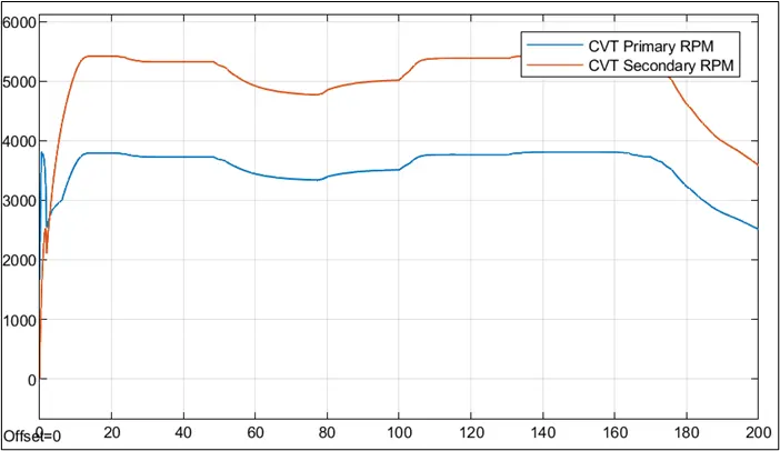
In above graph the rpm of CVT primary shaft for first few seconds was less and further it can be seen that the rpm was less as compared to the secondary shaft rpm by this it is clear that the rpm of the CVT output shat is more which increases the velocity of the vehicle.
*For the same model with the CVT ratio as shown in below figure the following output was obtained.*
CVT ratio along time.
The ratio for first few seconds was constant (3.5) and for time period 3 to 35 seconds was reduced to 0.5 and further it was kept constant and this ratio was fed to the CVT subsystem of the above ATV model.
Output for above shown CVT values:
The knobs were turned randomly to observe the changes in vehicle speed and CVT shaft rpm and the following results were observed.
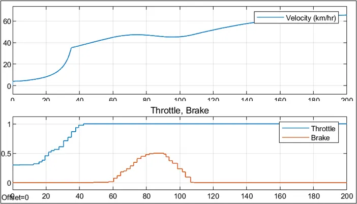
In the above graph the speed of the vehicle increases with increasing throttle and when brake was applied the speed was reduce to some extent. Then bringing brake to xero and throttle to max the gradual increase in speed can be observed.
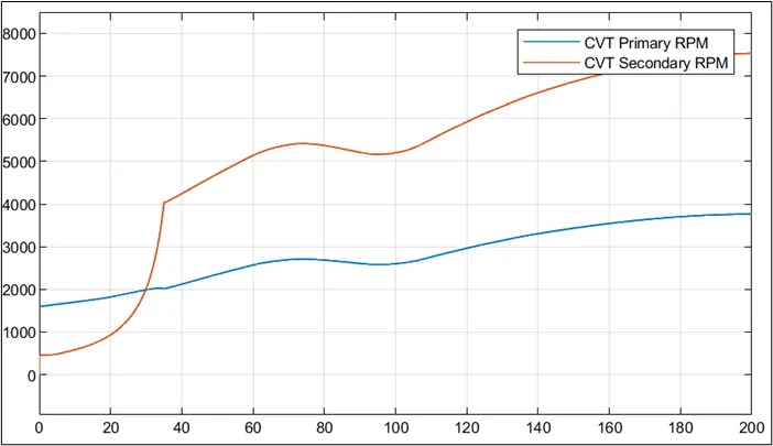
The graphical nature of RPM of CVT secondary shaft is similar to the speed of the vehicle, which increases with increase in throttle value and the rpm of primary shaft was less compared to secondary shaft.
3. BAJA ATV Model (mapped):
Simulink model:
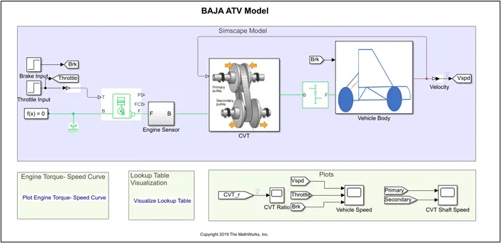
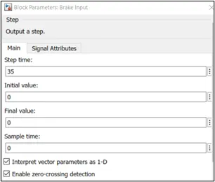
In this model the inputs Brake and throttle are produced using the step block and below snap shows the parameters defined for each input.
All the connections till the Engine sensor remain same as done in last two models, but CVT substation is quite different. The CVT subsystem has two inputs one from the generic engine through engine sensor and another is feed back signal fed from the output of the vehicle body, this can be understood better by looking inside the CVT sub system.
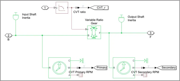
CVT sub system with lookup table.
Above image shows the blocks the CVT sub system consists of, where we can a 1D lookup table is used to connect the port ‘r’ of Variable ratio transmission (gear). The parameter block of 1D lookup table is shown in below image.
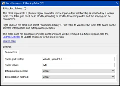
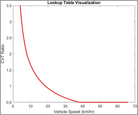
With the vehicle speed (feedback signal) obtained, the CVT ratio is adjusted by to the data of the Lookup table and below image shows the nature of CVT ratio along Vehicle speed. Where it was observed that the ratio was decreased from 3.5 to 0.5 for speed from 0 to 38km/hr and then the ratio was constant (0.5).
Output:
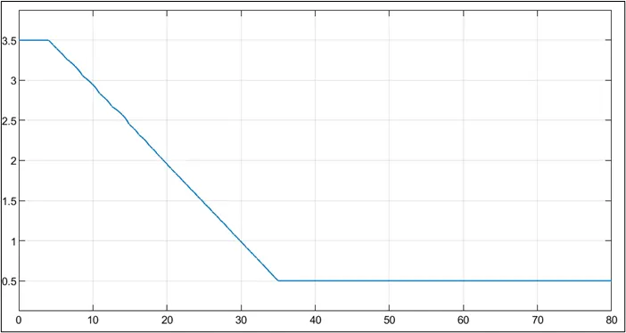
The above graph shows the CVT ratio (along Y-axis) along Time (along X-axis), where the ratio was constant for first few seconds and was reduced to 0.5 during time period from 4 to 35 seconds and then was constant.
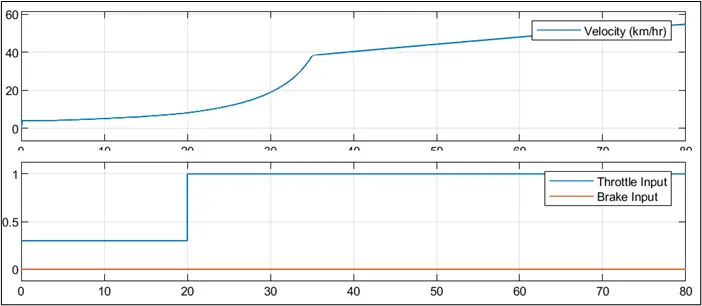
In the above graphs we can observe that during time period 0 to 20 second when throttle value was 0.3, there was a decent increase in the velocity from 0 to 8km/hr. But during time period from 20 to 80 seconds the throttle value was max and it can be seen the rapid increase in the velocity of the vehicle.
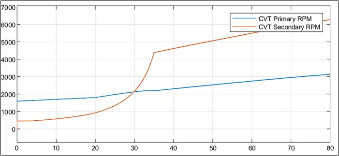
The above graph indicates the RPM value of the primary and the secondary shafts of the CVT.
4. BAJA ATV Model with dashboard (mapped):
Simulink model:
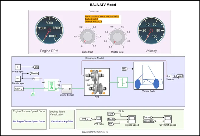
The above is the BAJA ATV mapped model with dashboard, everything in this model is same as BAJA ATV model mapped (without dashboard) except the dashboard and the input fed to the generic engine.
The dashboard consists of two Custom gauges (one for indicating the RPM at the engine sensor another for indicating the velocity of the vehicle body block) and two Knobs (one as Brake input another Throttle input). Using these knobs, the inputs are varied for this model and the corresponding out is recorded.
Output:
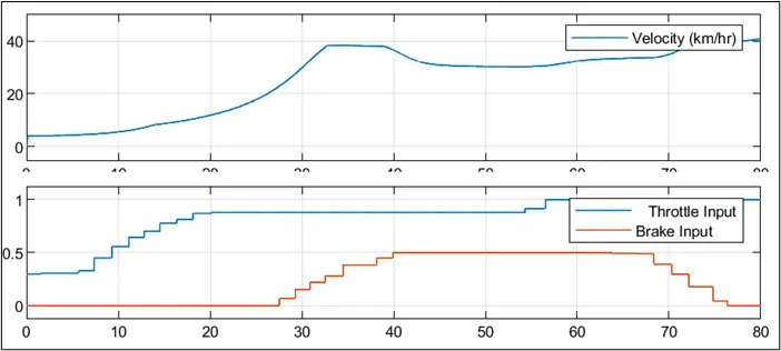
In the above graphs we can see that the speed of the vehicle with increase in the throttle value but when brake value is increased the velocity decreases to some extent.
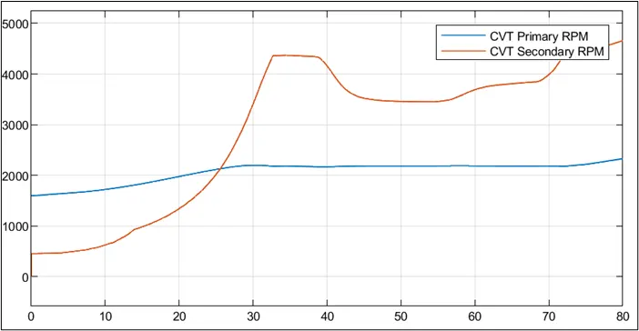
In the above graph it was observed that the rpm of primary shaft was less compared to the secondary shaft by varying the throttle value and brake value.
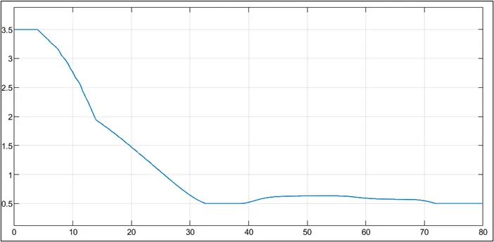
Above is the graph of CVT ratio (along Y-axis) v/s time (along X-axis) where the ratio obtained from the lookup table by referring the lookup table data.
References:
1. https://www.mathworks.com/matlabcentral/fileexchange/70576-baja-all-terrain-vehicle-atv-model
Conclusion:
- Study on BAJA ATV model was done and results were observed for different input values.
- The importance of using CVT in this model was understood.