Project

BAJA All terrain vehicle ATV model

Aim:

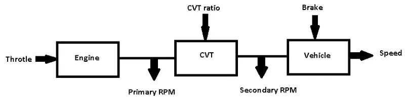
To model the BAJA all terrain vehicle ATV, that being used in the competition. This model helps to check the working for their designed vehicle for getting the characteristics for different throttle condition using simulink. For this model we need some prerequisite data from their designed vehicle. By this model anyone can simulate the effects of thorttle and brake as in actual situation. This simulation helps in conducting on various vehicle design for that we need just the data of the vehicle design.Using this model we can understand the how the engine provide the torque or speed for variable condition. Thus this model reduces the testing of actual system for different acceleration and brake input applied at different instant.

Introduction

The Baja SAE Competition originated at the University of South Carolina in 1976, under the supervision of Dr. Harit Mehta . Only 10 teams took part in the very first race. Since that time, the competition has grown to become a premier engineering design series with over 110 university teams participating in each race.

Dynamic Events are usually held on the final two days of competition. The first dynamic day includes the following events:

1. Acceleration
2. Hill Climb or Traction Event
3. Maneuverability
4. Specialty Events (Rock Crawl, Mud Bog, and Suspension).
5. An endurance race

The acceleration event is a measure of a vehicle's acceleration. The event is a 30.48 m (100 ft) or 45.72 m (150 ft) straight run from a standing start. The faster the time the more points the team will score. Every team can make two attempts with the best time counting for score. Vehicles with acceleration times that are more than 1.5 times that of the fastest vehicle will not receive a score for this event.

Hence this modelling only look after the characteristic of the vehicle while accelerating and braking. Accelerator is given through the throttle input and braking by brake input.

Prerequisite:

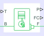
• Engine used in the vehicle along with speed vector, torque vectore, engine inertia etc.
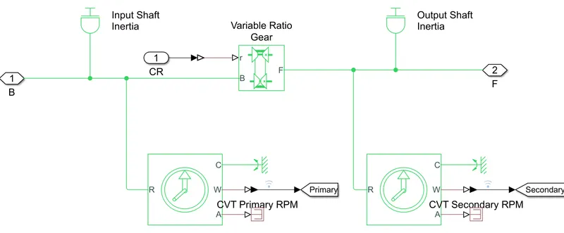
• CVT-Continuously Variable Transmission- A continuously variable transmission is an automatic transmission that can be change without use of clutch, through a continuous range of gear ratio. But in the other transmission provides limited number of gear ratio with fixed value. This Transmission helps engine to run at constant rpm while vehicle varies its speed and torque requirements.
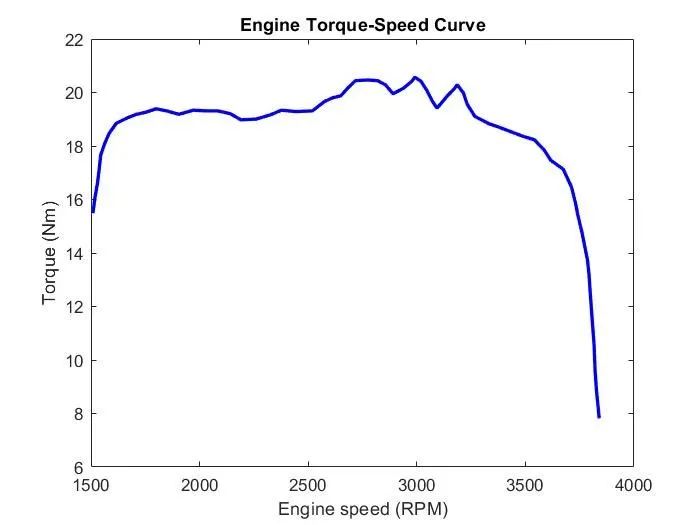
• Engine-Torque v/s Speed curve.
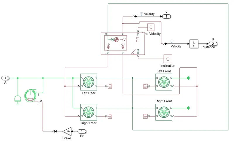
• Vehicle body dynamics(weight of body, tires, drag).

Difference in Modelling:

Model CVT ratio Controlled Thorttle Break Controlled

1. Predefined values No Constant Constant Signal Builder
2. Predefined values No Variable Variable Dashborad Knob
3. Lookup table Engine RPM Constant Constant Signal Builder
4. Lookup table Speed Of Vehicle Constant Constant Signal Builder
5. Lookup table Speed Of Vehicle Constant Constant Step Signal

Description:

Model 1:

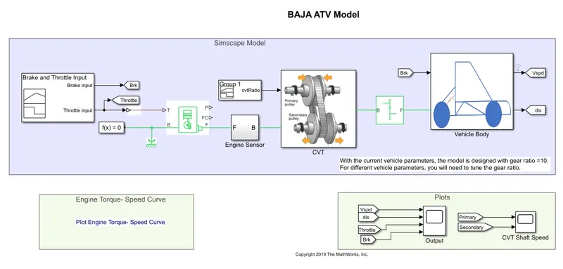
In this model Engine feed with throttle input and to the tyre brake input. CVT ratio build using signal builder. CVT is continuously varied as defined below. By this get the response of the single valued of throttle input at inital(start) instant.

Model 2:

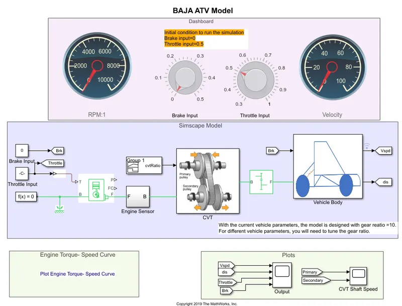
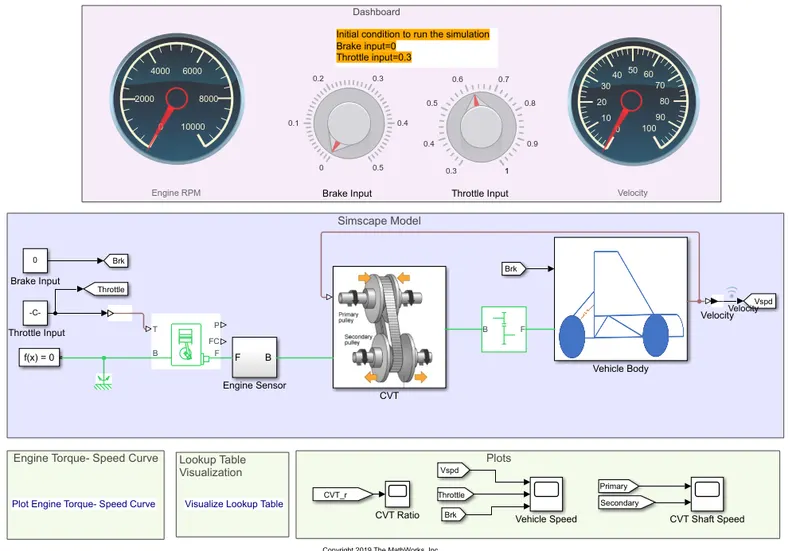
In this model same CVT ratio is feeded but to analyse the effects due to the different throttle input by continounsly wrt time. From this get the characteristics of the vehicle for different throttle value that can be varied using the dashboard knob.

Model 3:

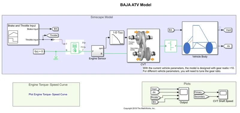
In this model CVT ratio is feeded using the lookup table and that lookup table is defined by the rpm of engine. As if in first case to analyse the constant values of throttle input, similarly here to analyse the single value is given but the throttle

Model 4:

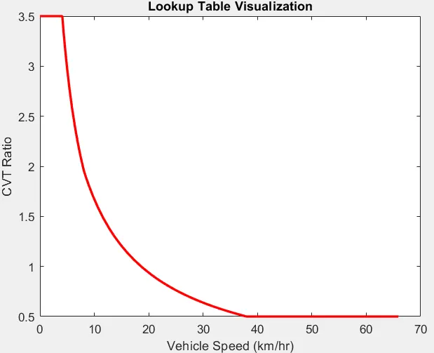
In this model CVT ratio is define using vehicle velocity, the vehicle velocity is feeded to the physical system lookup table and that provides the CVT ratio for the present velocity of vehicle. Ans also constant throttle is applied using step signal.

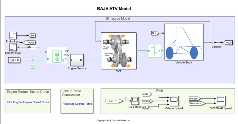
Model 5:

Similarly to model 4 CVT is controlled by the look up table wrt velocity of vehicle. To analyse the contuonus throttling control is given through dashboard knob.

Result:

Model 1:

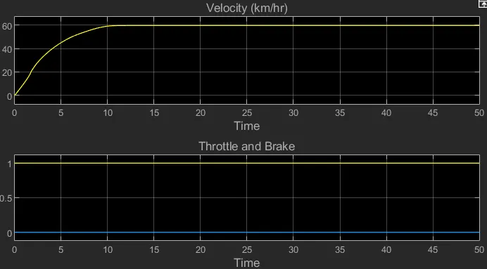
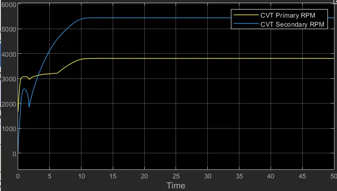
As the throttle given of 0.5 to the engine the rpm of engine(i.e Primary rpm) due to the initial inertia rpm left constant after some time engine gains energy the rpm raises. But on secondary side of CVT due to variable transmission even though constant engine rpm given due to the load torque requirement speed is reduced as the vehicle gains the achieve the speed over torque along with secondary rpm also increase. Hence this concludes the effects of constant throttle on the vehicle speed. Even if the throttle varied to 0.8. As compare to the throttle of 0.5, throttle 0.8 will provide the max velocity in less time. By this we can compare the results and selection of rate of the acceleration required and also for every different values throttle how the engine able reach its max rpm.

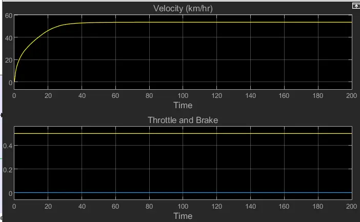
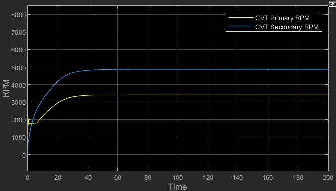
Figure Reaction of the system due to throttle 0.5

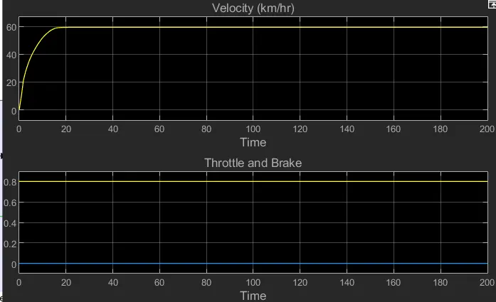
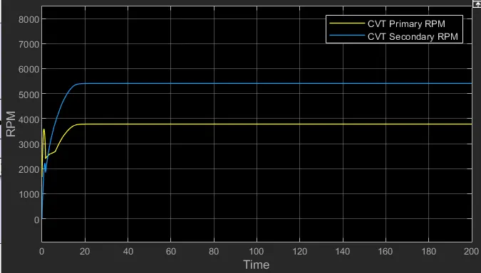
Figure Reaction of the system due to throttle 0.8

Model 2:

As we saw in model 1 one throttle given and velocity is analysed. But in practical this wont be happen once accelerator is pressed their might be situation that to vary the throttle for that we need to have the option to analyse the system for some period along with variable throttle as below.As we see the throttle varies engine rpm, output of the cvt and velocity varies continuously depending how much throttle given and this is dynamic change. And also if closly observed that even if throttle increase the engine rpm wont cross its max rpm but the cvt output increase where the gear is increasing. Hence we can see the action of variable transmission. This dashboard acts the peddle as in the practical scenario. Hence we can study the nature of the vehicle while throttle is continuously varied.

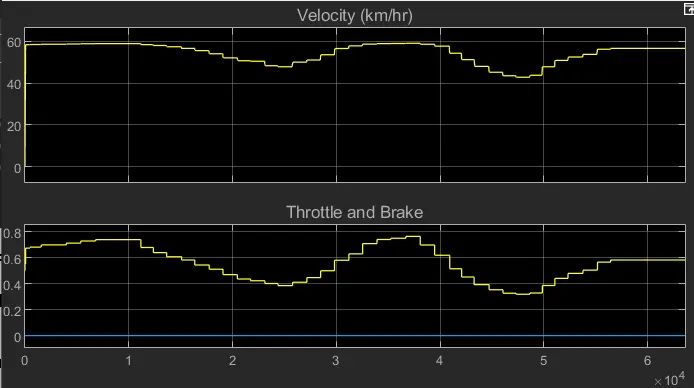
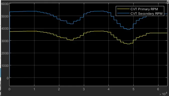
Model 3:

As we see from the above two model we selected only changing the throttle for some defined CVT ratio for all running period. But now using lookup table wrt to engine rpm we are controlling the cvt ratio. As we seen below constant throttle is given to analyse the change in CVT ratio from the engine rpm. So we can analyse only the CVT ratio here. Even though the throttle is constant but engine rpm has two phase of change. Although the engine rpm is changing the CVT output doesnot have the imact on that it has smooth surface as of in the first model. To develop the lookup table we need to have the breakpoints of the graph. For the breakpoints that was directly taken from the practical output results.

Model 4:

As in the above model to run the lookup table we need to have the practical test result. So here we use the simulation result to develop the lookup table for that we need to run previous test and log the cvt and velocity data. Using this data lookup table is analysed using matlab script. After getting the lookup table that lookup table take as reference as the velocity of the vehicle varied the cvt ratio is also varied. But for the only give data the cvt ratio are created for other than logged data the result will be zero.

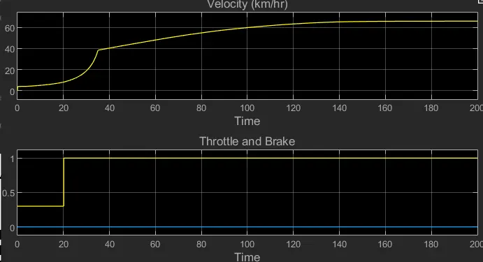
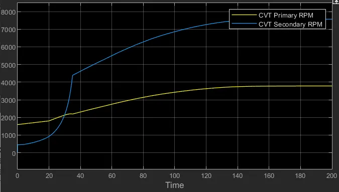
As we see that the throttle given after 20sec that imapcts on the engine rpm. But the output of cvt doesnot get much affected it only get affected due to the change in cvt ratio. That because the cvt ratio is set to get those output such that even their is low speed in the engine cvt can able to build the torque such that the vehicle attens the max speed.

Model 5:

All the lookup table models are tested only for the on instant change but that not happens in practical scenario. So we need to get back those dashboard into the previous model such that we can analyse all the change over long period. Even we able conclude that for every action given by the driver the velocity will be varied accordingly the cvt will control its ratio.

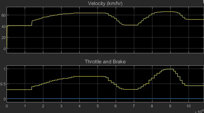
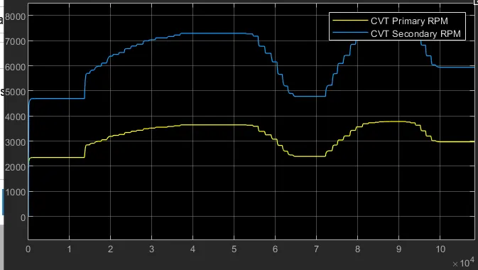
By this final output the total system able to react to the given throttle and accordingly the cvt ratio also being controlled. All the five models are the steps to achieve the final output that acts exactly by the vehicle in the practical scenario. These five model are helps us how to build the practical system. i.e

1. First we need to classify the control pramater and internal parameter. Also the dependent and independent parameter.
2. Then analyse only by changing the each control parameter on internal parameter
3. Then before implement the dependent and independent such that we get we need to sum up all the reaction due to control parameter.
4. Final building the complete system result in complete simulation of the full fuctional practical system