Project 2 Thermal modeling of battery pack

Aim - Thermal Modelling of a Battery Pack for a 10 cell series lithium ion battery model

Objectives -

• Simulate the thermal effects.
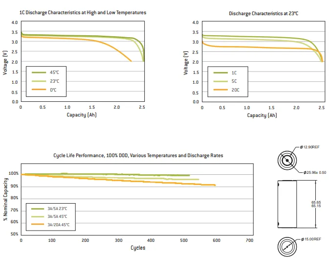
• Compare life cycle performance at various temperatures, charge & discharge rates.

Theory -

Introduction -

The performance and life-cycle costs of electric vehicles (EV) and hybrid electric vehicles (HEV) depend inherently on energy storage systems such as batteries. Battery pack performance directly affects the all electric range, power for acceleration, fuel economy, and charge acceptance during energy recovery from regenerative braking.

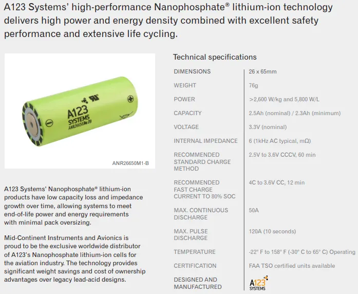
ANR26650M1-B Nanophosphate lithium iron phosphate (LiFePO4) datasheet used for this project:

Convection -
Most of the commercial battery thermal management systems rely on convection as controllable heat dissipation methods. Depending on whether the surrounding media is actively driven or not, the mechanisms is called forced or natural convection. The cooling or heating effect can be realized using gaseous or liquid media (e.g., air or water). The basic correlations for conductive heat transfer are given in Equation (13.2). Hereby labels the average convection coefficient, being a function of the Nusselt, Reynolds, and Prandtl number of the flow field.

Working of simulink model:

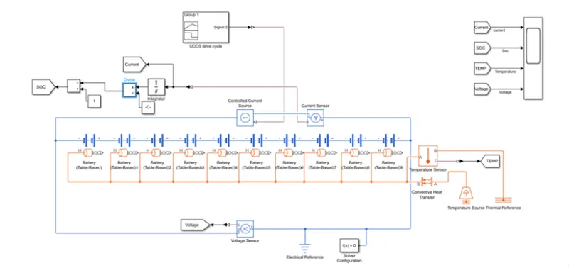
• Firstly we took the table based battery and then made it as instrumented and show thermal port and rest all the parametres as default,we are using matlab default data not from anyu data sheet.And then we conected 10 such cell in series with same configuration.so the voltage across the pack is multplied by 10 and the capacity is same through out the pack.
• Now we conected a voltage sensor to the 2 torminal negative from the first and positive from the last and a goto block is conected through ps to simulink converter to the voltage sensor to take the output voltage and a from block is connected to the scope to recieve the voltage signal.
• The controlled current source is connect to the battery to take the current from the battery and there a current sensor is connected to sense how much current is drawn from the battery and that current is again connected to go to block through ps to simulink converter and a from block is there to recieve the signal and give it to the scope.
• The same current is now integrated through integrator block and then divided by total capacity of the pack which is 27Ah(27*3600) to make it in ampre second,that is now substracted from one so that it will give the soc of the battery. and a goto block is conected to take the output SOC and a from block is connected to the scope to recieve the SOC signal.
• A signal builder is taken to give the input to the controlled current sensor and UDDS drive cycle data is used in the form of current with respect to time.
• Now at the thermal port the temperature source is connected to give the external temperature and it is not connected directly it is connected through the convective heat transfer block so that the area of contact we increase and as we give the temperatue input to the temperature source block. There a temperature sensor is connected to sense the temperature of thr battery pack and one port is connected to thermal reference.
• The output of the temperature sensor is connected to goto block throught ps to simulink converter block and a from block is connected to the scope to take the temperature signal to the scope.
• finally a electrical reference is connected the the electrical side of the model for ground and also a solver configuration is connected.
• And we run the simulation for 1369sec as the input current is only for the 1369 sec if we go beyond the graph will so constant because no load current is drawn from it.

Simulink Model -

Blocks used -

1. Battery (Table based) - This block models a battery based on tabulated characteristics as functions of state of charge (SOC) and optional temperature (T).

2. Electrical Reference - electrical grounding.

3. Thermal Reference - thermal grounding.

4. Scope - To view the output graphs.

5. Temperature Sensor - sensing temperature.

6. Convective Heat Transfer - This block models heat transfer in a thermal network by convection due to fluid motion. The rate of heat transfer is proportional to the temperature difference, heat transfer coefficient, and surface area in contact with the fluid.

7. Temperature Source - This block represents an ideal energy source in a thermal network that can maintain a constant absolute temperature at the port regardless of the heat flow rate.

8. Controlled Current Source - The block represents an ideal current source that is powerful enough to maintain the specified current through it regardless of the voltage across it. The output current is I = Is, where Is is the numerical value presented at the physical signal port.

9. Voltage Sensor - The block represents an ideal voltage sensor, that is, a device that converts voltage measured between any electrical connections into a physical signal proportional to the voltage.Connections + and - are conserving electrical ports through which the sensor is connected to the circuit. Connection V is a physical signal port that outputs voltage value.

10. Signal Builder -

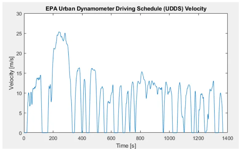
The US FTP-72 (Federal Test Procedure) cycle is also called Urban Dynamometer Driving Schedule (UDDS) or LA-4 cycle (CFR 40, 86. App. I) [2656]. This cycle should not be confused with the UDDS schedule for heavy-duty vehicles. The cycle simulates an urban route of 7.5 mi (12.07 km) with frequent stops. The maximum speed is 56.7 mph (91.25 km/h) and the average speed is 19.6 mph (31.5 km/h).

11. Integrator block -

12. Solver configuration - Defines solver settings to use for simulation.

13. Goto Block - Send signals to From blocks that have the specified tag.

14. From block - Receive signals from the Goto block with the specified tag.

Simulation O/P Graph :

Case #1 :

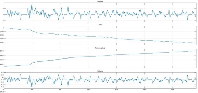
• Here all the default value is given to the the blocks and the simulation results are here.In the first graph the current drawan is there and it is same as the the drive cycle because we used it same and se there the maximum vaue is goes upto 8 and the minimum is -5 which shows of charging regen braking.
• The second graph is of soc which is in the decreasing form but in linear, it is some time charging and some time it is discharging as per the current goes positive or negative.it starts from 1 which is full charge after the whole simulation it is at 0.992 which is aproxx full.
• Third graph is Temperaturewhich is default one i didn't made any changes,so it is increasing from 298.1 to 298.5 which not much rising.
• Finally at the last it is voltage fluctuation with respect to time and it starts from 41.9v and ends at same 48.9 and in between it is increasing and decresing as the battery is charge or discharge or as per the current drawn or supplied.The max voltage drawn is42.2v and minimum is 41.2v.

Case #2 : Now we are changing the temperature data

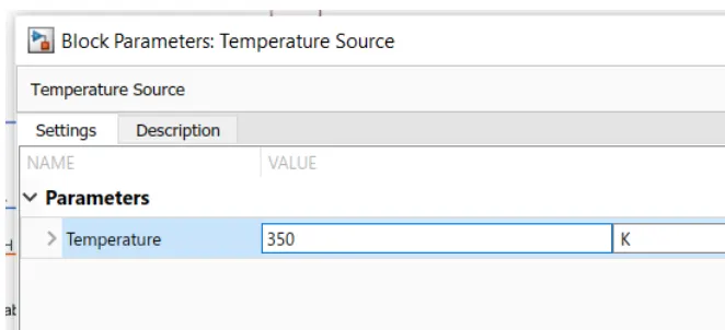
Here from the temperature source we change the temperature to 350k.

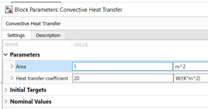
And in convective heat transfer,the area we made from 1e-1 to 1m^2.

lets se the result the simulation time and rest all parametres are same.

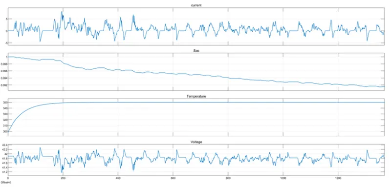
• Here we can see the first graph of current is same because we didn't made changes on the load side.The graph is same as above.
• The second graph is soc where also we are not seing any difference because th runing time is very low we can se any changes here.
• The 3rd graph which is temprature with respect to time here it is changed like first it starts from 300 and it increases upto 350 and hen it goes constant after 200 sec.So yes we have seen the hude difference from the prvious one.
• The last is voltage graph which is also very much similar to previous one.

Case #3 : Now i am change agiain the temperature parametre to negative lets see what is happening:

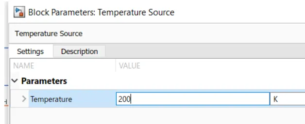
here we made the temperature to 200k which is aproxx equal to -73.15°C

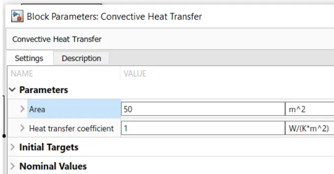
And the area in the convective heat transfer made to 50m^2,and th coefficient to 1.

Lets see the result:

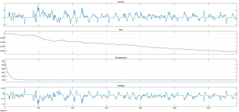
• Here as above the current is same because no changes made on load side.
• The second graph is soc as i told previous where also we are not seing any difference because th runing time is very low we can se any changes here.
• The 3rd graph which is temprature with respect to time here it is changed like first and second it is different totaly starts from 300 and it decreases down upto 200 and then it goes constant after 200 sec.So yes we have seen the hude difference from the prvious one and the first one.

Conclusion -

Due to temperature difference the cycle of charge dicharge is not much varriying here but in real life it must be vary and the temperature of the battery changes by variying the outside teemperatur suplied.

The flow of heat is decreased at constant and minimum temperature that is 309 k for different temperature based.
Based on different temperature we will see changes in conduction and convection.
There is slightly changes in cyclic charge and discharge of cell which I fixed at 50A as peek amplitude.
As I set fault in cell-5 and we can see that there is lots of fluctuation and temperature rise in cell-5 as compared with other cells connected in series.
SOC for all different temperature are same, there is no changes in SOC.