Project 2 Thermal modeling of battery pack

Project - Thermal Modeling of a Battery Pack

Aim: To model a thermal model of a battery pack

Objective: For a 10 cell series lithium ion battery model, simulate the thermal effects and compare life cycle performance at various temperatures, charge & discharge rates using MATLAB.

Solution:

A. For the project, we have to model a battery pack with 10 cells in series and simulate its thermal effects. The battery pack can be built as:

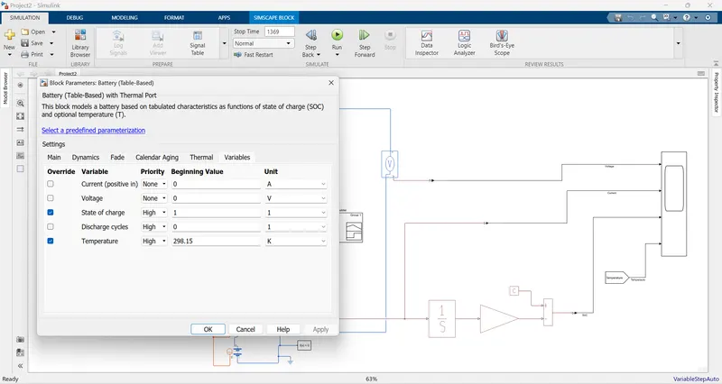
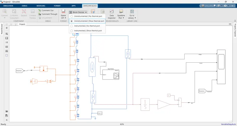
1. Add a battery(table-based) from Simscape -> Electrical -> Sources. Click on the battery, look for the simscape block window in the toolbar. In it, go to block choices -> Select 'Uninstrumented|Show Thermal Port'. This will enable the thermal ('H') port in the battery. Double click on the battery pack to view its parameters. Go to the varibles section and select 'State of charge' and 'Temperature' variables. Now create 9 more copies of the battery and connect the negative of one to the positive of another. This creates a battery pack with 10 cells in series.

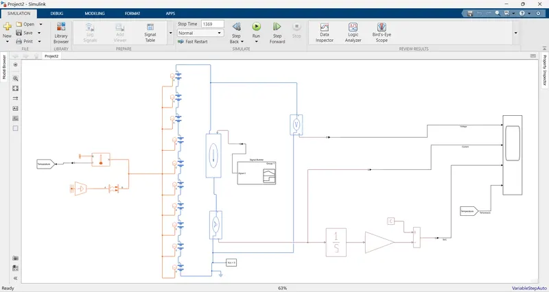
2. Now group the 'H' ports of all the battery packs. Add a 'convective heat transfer' block from Simscape -> Foundation Library -> Thermal -> Thermal Elements. Also, add a 'controlled temperature source' block from Simscape -> Foundation Library -> Thermal -> Thermal sources. Now connect the 'A' port of the heat transfer block to the temperature source and the B port to the grouped 'H' port of the battery pack. We have to measure the temperature change of the battery; for it, we will require a temperature sensor. To fetch it go to Simscape -> Foundation Library -> Thermal -> Thermal Sensors. Connect the 'A' port of the temperature sensor to the 'B' port of the heat transfer block ,whereas, the 'B' port of the sensor should be connected to a thermal reference. The 'T' port would be the output port. Connect a PS-Simulink converter to the 'T' port.

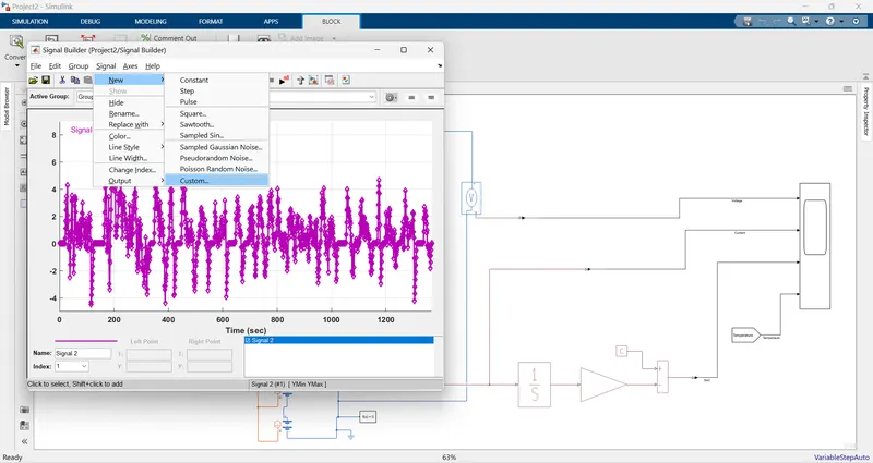
3. Having done all this, we need to connect some load to the pack to discharge it and view the thermal effects. For it, we take into consideration the UDDS drive cycle. The drive cycle can be obtained from internet. A drive cycle is the plot of speed vs time. To use these values in our model, we need to convert them to current values. After converting the speed values to current values we can use them in a Signal builder block. To fetch the Signal builder block go to Simulink -> Sources. In the block, load the drive cycle and the output of the block shall be connected to the controlled current source. To load the values in Signal builder we have to follow: Signal -> New -> Custom -> Copy paste the time and current values in square brackets.

4. We can't connect the signal builder directly to the battery as it would make no sense to the battery. Hence, we get in a controlled current source block from Simscape -> Electrical -> Electrical Sources. We connect the block such that the arrow point towards the negative terminal of the last cell in the assembly. The signal builder block is connected to the source port of this source block.

5. Now, the output of the system needs to be viewed to draw some inference about the characteristics of the system. We require to view the voltage, current, SoC and temperature change parameters of the battery pack.

a. To view the voltage, we connect a voltage sensor across the pack.

b. To view the current, we connect a current sensor through the pack.

c. To calculate the state of charge, we shall use the Coulomb counting method. For it, we integrate the current values over the simulation time and divide it by the max battery capacity (3600 because the integrated values are in A*s whereas the pack capacity is in A*h). By doing this, we obtain the depth of discharge, i.e. how much charge has been removed from the battery. When we subtract it form 1, we get the SoC of the battery, i.e. the amount of charge left in the battery.

e. The temperature values can be obtained from the 'T' port of the temperature sensor.

All these can be viewed in a scope sourced from Simulink -> Sinks.

The model:

Outputs:

1. Firstly, for the temperature source at default value of 293.15 K, the outputs are as:

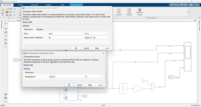
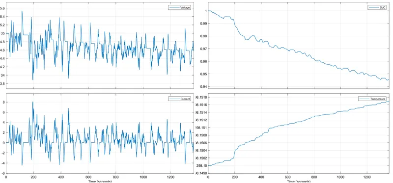
As the UDDS cycle is representative of urban driving conditions, there are frequent starts and stops in the cycle. This leads to a fluctuating nature of the current and voltage graphs. The positive current represents discharging. while the negative value represents charging through regenerative braking. The SoC curve also shows a rise and fall behaviour corresponding to the cycle but overall the SoC of the pack falls from 100% to about 94.5%. Our source is at a temperature of 293.15 K, while our pack is initially at 298.15 K. As the pack is discharging, the temperature of the pack rises because of the chemical reactions taking place inside the pack. However, because of the temperature source, the rise in temperature is within limits.

2. For the temperature source at 273.15 K:

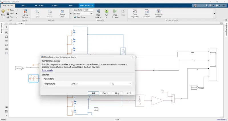
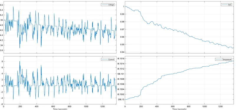
When the temperature of the source is reduced, the final pack temperature also reduces marginally, signalling some cooling.

3. For the temperature source at 313.15 K:

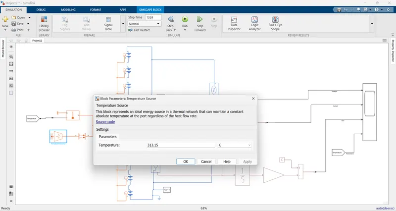
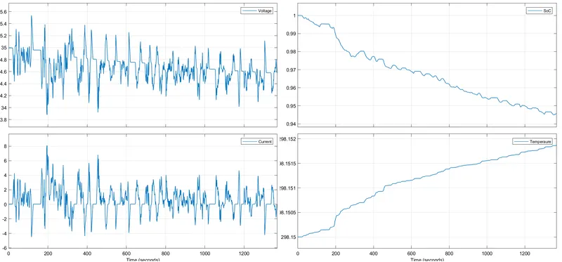
Now, when the temperature of the source is increased, the final pack temperature rises, singalling some form of heating.

4. Now lets see the effect of change in area on the thermal effects. Firstly, for the default area of convective heat transfer block of 1e-4 m2, the temperature is as shown in point no. 1. If the area is increased, with the temperature being kept at the same level, the results are as:

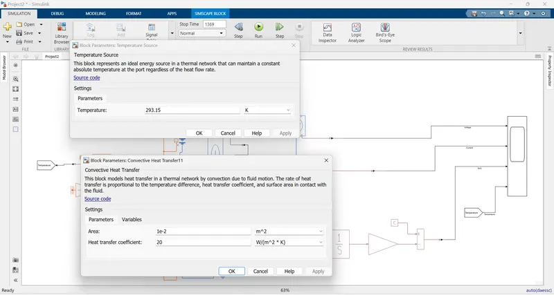
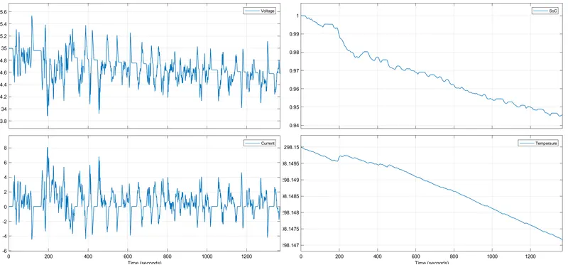
With an increase in the area of contact, the final pack temperature reduces. This could be helpful in the cooling of the battery pack.

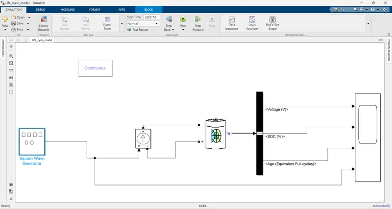
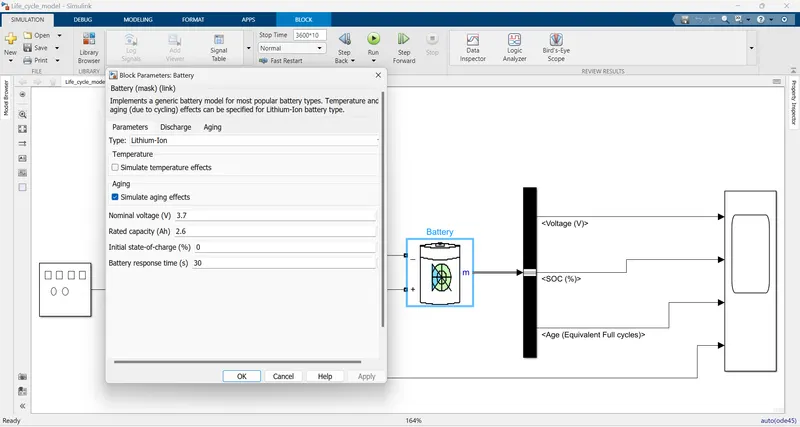
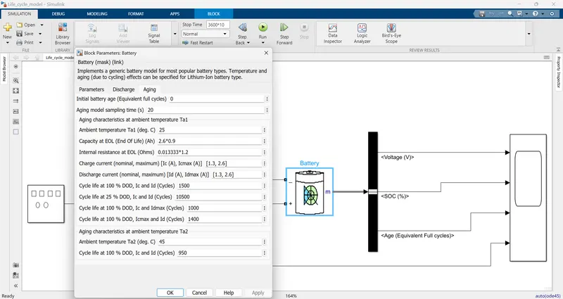
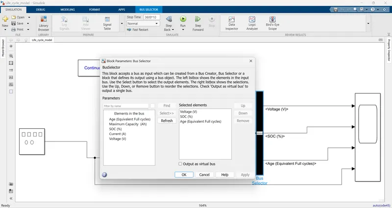
B. For the second part of the question, we have to build a separate model as the earlier model doesnot have provisions to calculate aging of the pack. To build the model, we will source a battery and a constant current source from Simscape -> Electrical -> Specialised Power Systems. The battery specs are set according to the cell parameters for 18650 cell. As an input to the system, we shall apply a square waveform representing charging and discharging corresponding to positive and negative curves respectively. Then by introducing a bus selector, we can view the desired parameter outputs of the cell. Accordingly the model is built as:

Outputs:

1. For a C-rate of 1C the outputs are as:

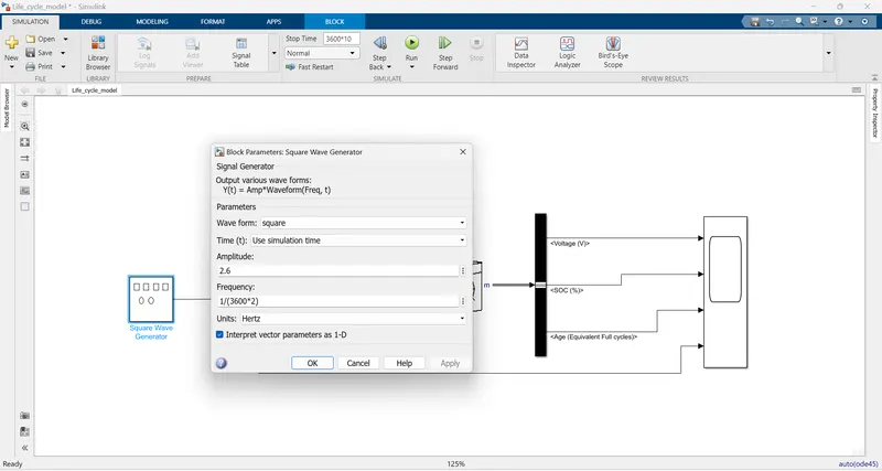
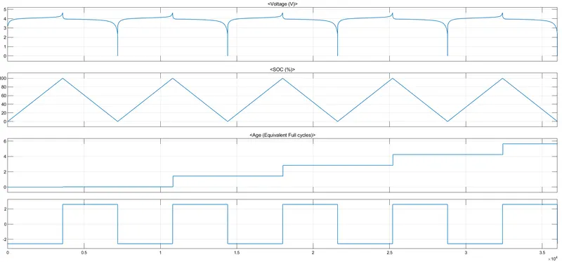
For a C rate of 1C, the cell charges upto 100% and discharges to 0% in a complete cycle. The cell loses about 6 life cycles out of its entire rated life cycles at this rate of charging/discharging.

2. For a C-rate of 0.5C:

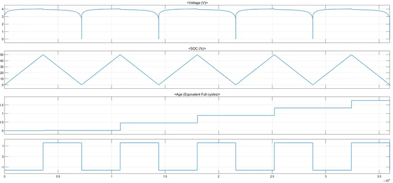
For 0.5C, the cell charges only upto 50% and discharges thereafter to 0%. This indicates that at 0.5C, the cell requires more time to charge completely. But at this rate, the cell loses only about 2 life cycles as compared to the 1C rate, for the same number of charge/discharge cycles.

3. For a C-rate of 2C:

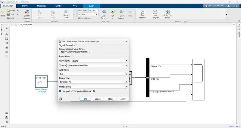
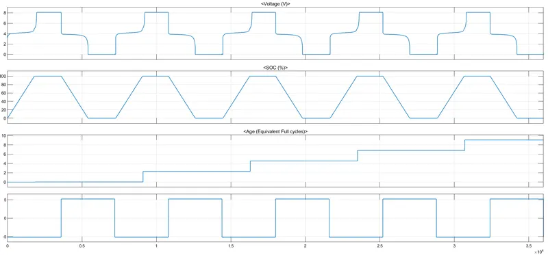
For a 2C rate, the cell charges upto 100% at a faster pace than 1C rate. At this rate, the cell loses about 9 cycles of its total life cycles for the same number of charge/discharge cycles. This indicates that the cell should be charged/discharged at its rated C-rates as much as possible, to improve the life of the cell.

References:

MATLAB Documentation

!!! Thank You !!!