Project 2 Thermal modeling of battery pack

Objective:

Thermal Modelling of Battery Pack

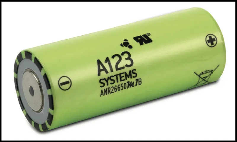
Cell: ANR26650M1-B

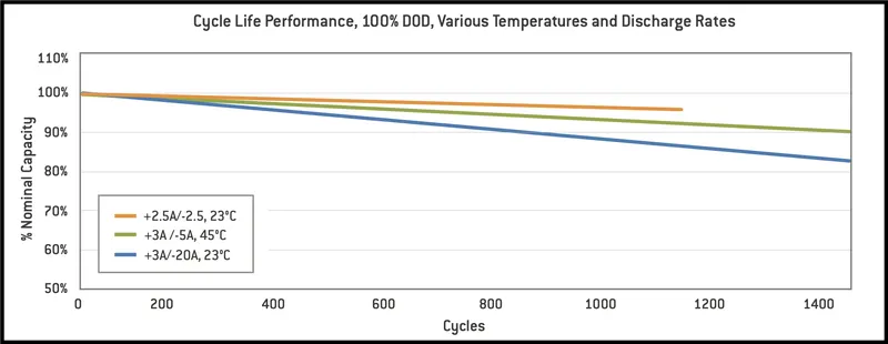
For a 10 cell series lithium ion battery model, simulate the thermal effects and compare life cycle performance at various temperatures, charge & discharge rates using MATLAB.

Theory:

Li-ion cell(ANR26650M1-B):

A123’s high-performance Nanophosphate® lithium iron phosphate (LiFePO4) battery technology delivers high power and energy density combined with excellent safety performance and extensive life cycling in a lighter weight, more compact package.

For outstanding cycle life, stable float reliability this cells are suitable for a wide variety of power, pulse and stand by applications.

Nanophosphate battery technology offers thermal stable chemistry, fast charging, consistent output, low capacity loss over time.

It provides extremely safe conditions for while meeting most demanding customers requirements.Multiple layers of protections are employed on chemistry, cell and system level to achieve an energy storage solution with superior safety.Our cells have low capacity loss and impedance growth over time as well as high usable energy over a wide state of charge (SOC) range, allowing our systems to meet end-of-life power and energy requirements with minimal pack oversizing.

Applications:

COMMERCIAL SOLUTIONS

Advanced lead acid replacement batteries for:

+ Datacenter UPS
+ Telecom backup
+ITbackup

+ Autonomously guided vehicles (AGVs)
+ Industrial robotics and material handling equipment + Medical devices

GOVERNMENT SOLUTIONS

+ Military vehicles
+ Military power grids + Soldier power
+ Directed energy

GRID SOLUTIONS

+ Frequency regulation
+ Renewables integration
+ Reserve capacity
+ Transmission and distribution

TRANSPORTATION SOLUTIONS

Hybrid, plug-in hybrid and electric vehicle battery systems for:

+ Commercial vehicles
+ Off-highway vehicles
+ Passenger vehicles

10 cell series lithium ion battery model:

Blocks needed in making simulink model:

• Battery (Table based)

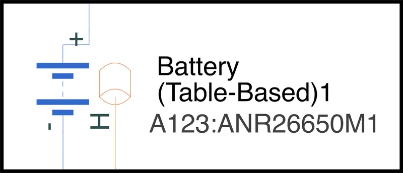
This block models a battery based on tabulated characteristics as functions of state of charge (SOC) and optional temperature (T).

Here we made the ports to instrumented and show thermal port.

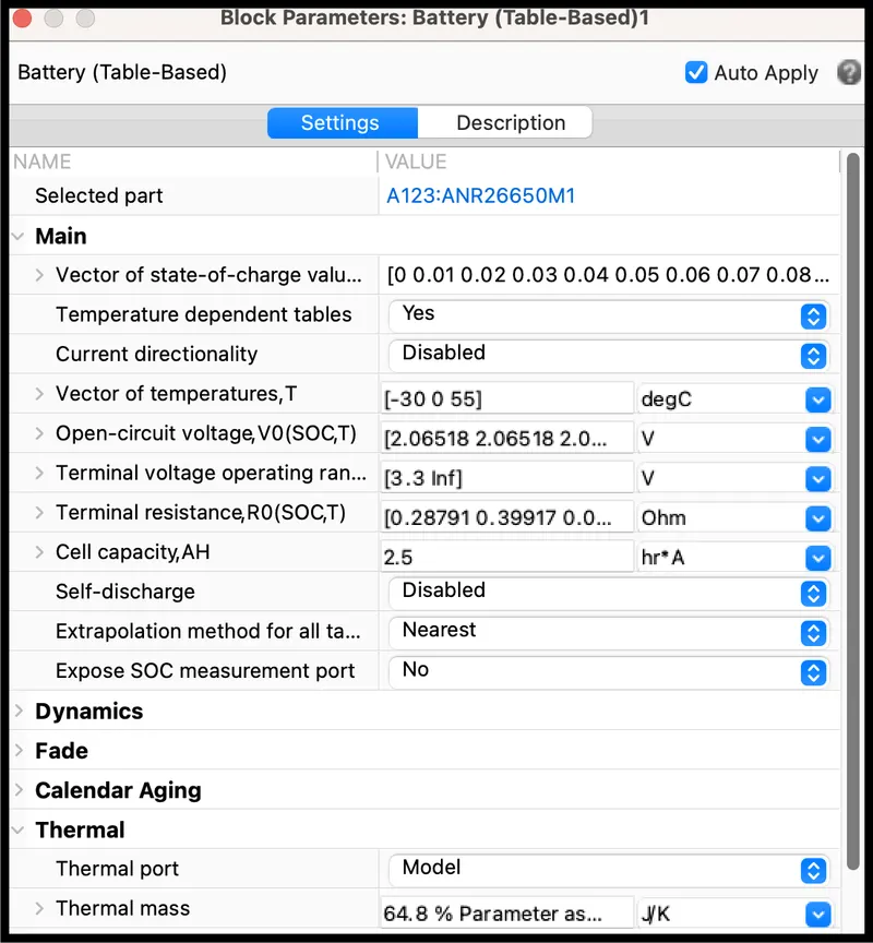
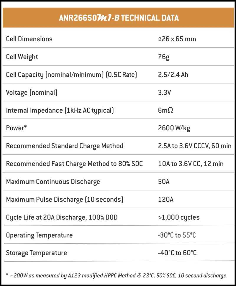
The thermal port is showing in the model. Nominal voltage 3.3 V battery capacity 2.5 Ah as per data sheet.

Here we made same 10 battery block with the parameters are same as default nothing to do any changes.

• Controlled Current Source

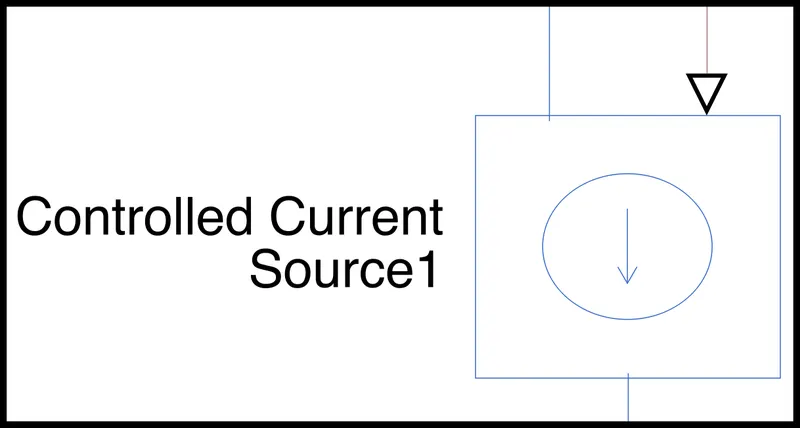
The block represents an ideal current source that is powerful enough to maintain the specified current through it regardless of the voltage across it. The output current is I = Is, where Is is the numerical value presented at the physical signal port.

• Current Sensor:

The block represents an ideal current sensor, that is, a device that converts current measured in any electrical branch into a physical signal proportional to the current.Connections + and - are conserving electrical ports through which the sensor is inserted into the circuit. Connection I is a physical signal port that outputs current value.

• Temperature Source:

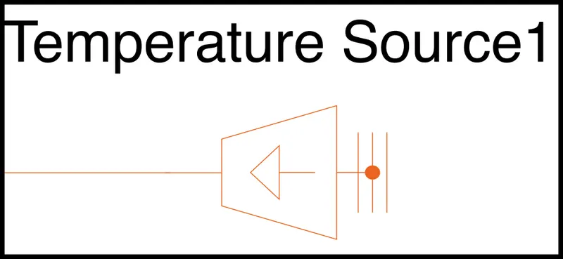
This block represents an ideal energy source in a thermal network that can maintain a constant absolute temperature at the port regardless of the heat flow rate.

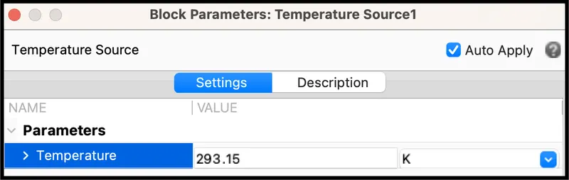
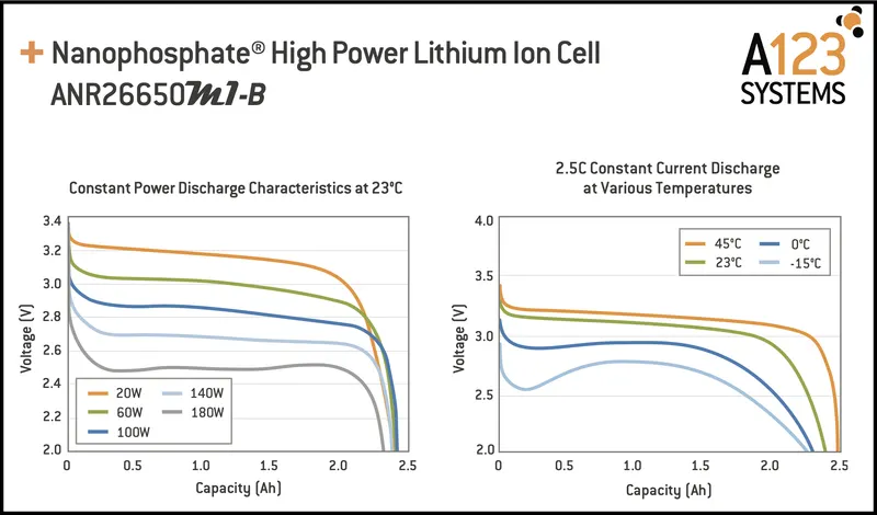
Here its default value is 293.15k, we are going to vary the temperature value to see the charge and discharge at various temperature.

• Temperature Sensor:

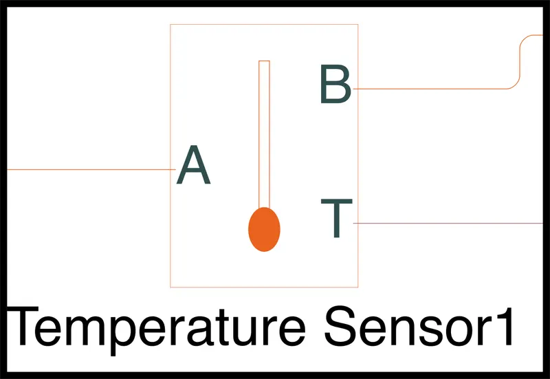
This block measures temperature in a thermal network. There is no heat flow through the sensor. The physical signal port T reports the temperature difference across the sensor. The measurement is positive when the temperature at port A is greater than the temperature at port B.

• Thermal reference:

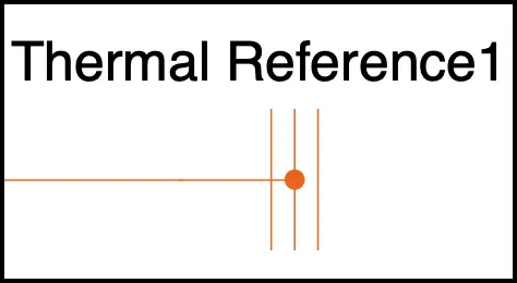
This block represents a reference point in a thermal network where the temperature is equal to absolute zero.

• Convective heat transfer block:

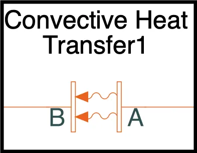
This block models heat transfer in a thermal network by convection due to fluid motion. The rate of heat transfer is proportional to the temperature difference, heat transfer coefficient, and surface area in contact with the fluid. The heat transfer coefficient can be either constant or variable. When the heat transfer coefficient is variable, specify it using the physical input signal at port K. If the heat transfer coefficient is variable, it remains at the Minimum heat transfer coefficient if the physical signal falls below this value.

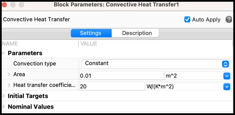
Here the area of contact and heat transfer coefficient is having default vlue but we shall change it at the time of simulation.

• Voltage Sensor:

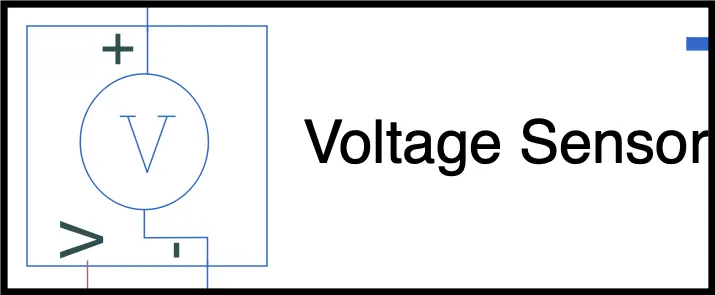
The block represents an ideal voltage sensor, that is, a device that converts voltage measured between any electrical connections into a physical signal proportional to the voltage.

Connections + and - are conserving electrical ports through which the sensor is connected to the circuit. Connection V is a physical signal port that outputs voltage value.

• PS Constant1

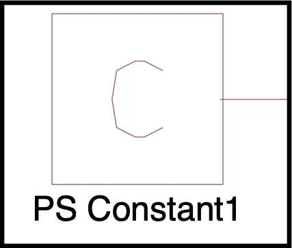
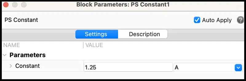
This block creates a physical signal constant:

y = constant as value set to 1.25 which is taken from data sheet discharge rate is 0.5C -applied constant load and Cell capacity 2.5 Ah.

The Constant parameter accepts both positive and negative values. The block output is a physical signal port.

• Electrical Reference:

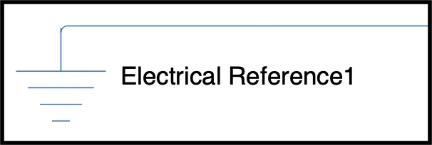
Electrical reference port. A model must contain at least one electrical reference port (electrical ground).

• Integrator block:

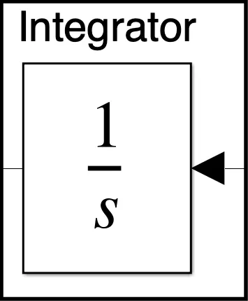
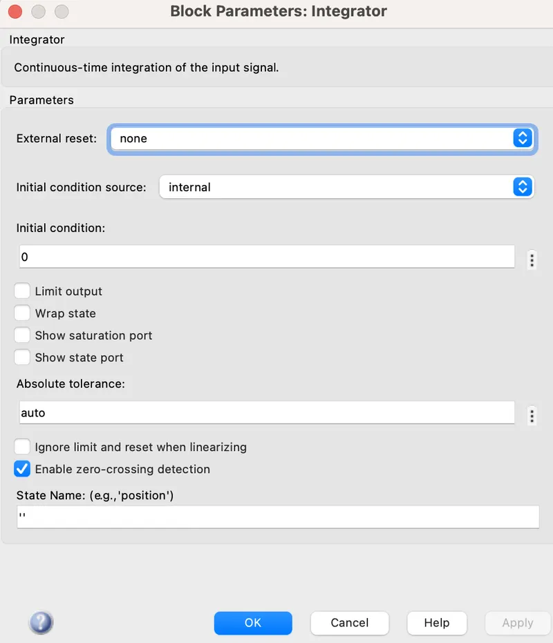
All the input parameters are same as default .

• Solver configuration:

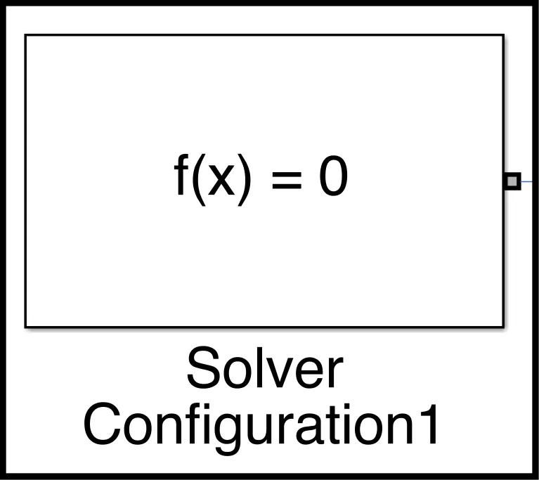
Defines solver settings to use for simulation. We kept as default settings.

• Goto Block:

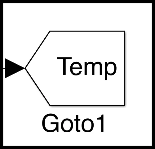
Send signals to From blocks that have the specified tag. If tag visibility is 'scoped', then a Goto Tag Visibility block must be used to define the visibility of the tag. The block icon displays the selected tag name (local tags are enclosed in brackets, [], and scoped tag names are enclosed in braces, {}).

• From block:

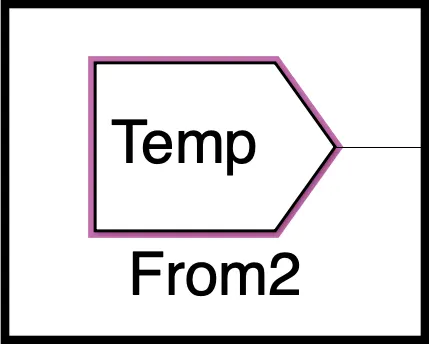
Receive signals from the Goto block with the specified tag. If the tag is defined as 'scoped' in the Goto block, then a Goto Tag Visibility block must be used to define the visibility of the tag. After 'Update Diagram', the block icon displays the selected tag name (local tags are enclosed in brackets, [], and scoped tag names are enclosed in braces, {}).

• Scope:

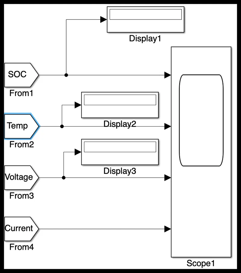
Show the results of the simulation in the form of plot.

• PS-Simulink Converter

Converts the input Physical Signal to a Simulink output signal.

Format of Simulink output signal matches the format of Physical Signal. 'Vector format' provides an option for outputting vector Physical Signals as Simulink 1-D arrays.

SIMULINK MODEL 10 Cells In Series -Constant Load Applied

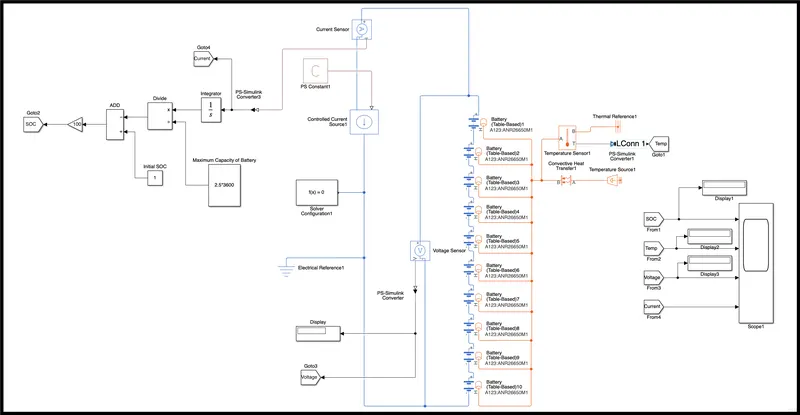
Working of simulink model:

• Initially we selected the table based battery and then made it as ANR26650M1and show thermal port and rest all the parameters as default, we are using data from ANR26650M1 data sheet.And then we connected 10 such cell in series with same configuration.so the voltage across the pack is multiplied by 10 and the capacity is same through out the pack.
• To check voltage across battery pack, we connected voltage sensor to the two terminal negative from the last and positive from the first. V output is connected through PS to simulink converter to the output voltage display and goto for scope namely Voltage as tag globally visible.
• The controlled current source is connect to the battery to take the current from the battery and there a current sensor is connected to sense how much current is drawn from the battery , using coulomb Counting Method and that current is again connected to go to block through PS to simulink converter and a from block is there to receive the signal and give it to the scope.
• The same current is now integrated through integrator block and then divided by total capacity of the pack which is 2.5Ah(2.5*3600) to make it in ampere second, that is now subtracted from one so that it will give the SOC of the battery. and a goto block is connected to take the output SOC and a from block is connected to the scope to receive the SOC signal.
• A Constant block is connected to controlled current source. It is acting like constant load applied to the battery pack with discharging maximum rate of 0.5C of battery capacity and battery capacity is 2.5 Ah though 10 cells connected in series.
• Now at the thermal port the temperature source is connected to give the external temperature and it is not connected directly it is connected through the convective heat transfer block so that the area of contact can increase or decrease. There a temperature sensor is connected to sense the temperature of the battery pack and one port is connected to thermal reference, it will help to measure temperature.
• The output of the temperature sensor is connected to goto block through PS to simulink converter block and a from block is connected to the scope to take the temperature signal to the scope.
• finally a electrical reference is connected the the electrical side of the model for ground and also a solver configuration is connected.
• And we run the simulation for 3600 sec as the input current is also for the 3600 sec .

Simulation result:

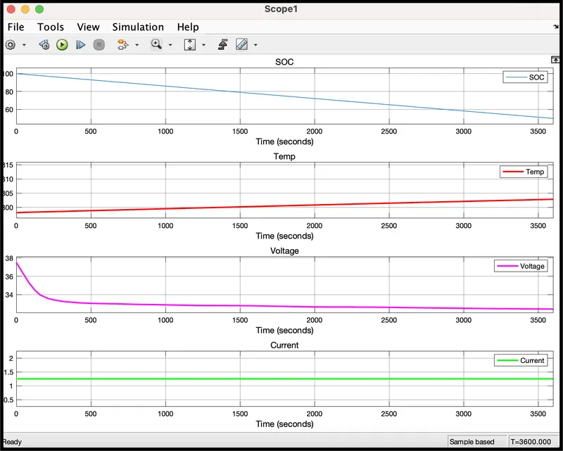
• Here all the default value is given to the the blocks and the simulation results are here.In the first graph the SOC drawn and it is same as the constant load.
• The SOC graph is decreasing form 100% but in linear, it is discharging as per the current goes negative.it starts from 100% which is full charge after the whole simulation it is at 50% which is half.
• Temperature graph which is default one I didn't made any changes, so it is increasing from 293.15 to 302.85584610773 which not much rising.
• Finally at the last it is voltage fluctuation with respect to time and it starts from 37.2 V and ends at 32.430926895749 V and in between it is decreasing as the battery is discharge as per the current drawn.

SIMULINK MODEL 10 Cells In Series -UDDS Applied

Working of simulink model:

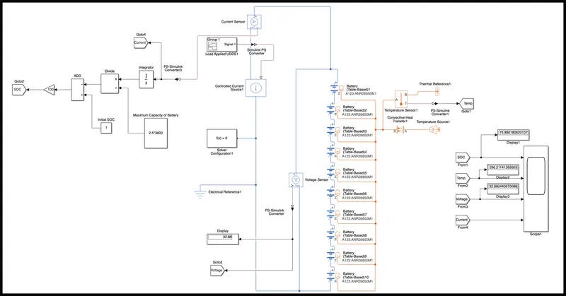
In this case used UDDS

• A signal builder is taken to give the input to the controlled current sensor and UDDS drive cycle data is used in the form of current with respect to time.
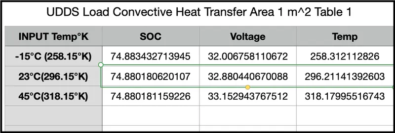
• Now at the thermal port the temperature source is connected to give the external temperature and it is not connected directly it is connected through the convective heat transfer block so that the area of contact we increase and as we give the temperature input to the temperature source block. There a temperature sensor is connected to sense the temperature of the battery pack and one port is connected to thermal reference.
• The output of the temperature sensor is connected to goto block through ps to simulink converter block and a from block is connected to the scope to take the temperature signal to the scope.
• finally a electrical reference is connected the the electrical side of the model for ground and also a solver configuration is connected.
• And we run the simulation for 3600 sec as the input current is only for the 3600 sec if we go beyond the graph will so constant because no load current is drawn from it.

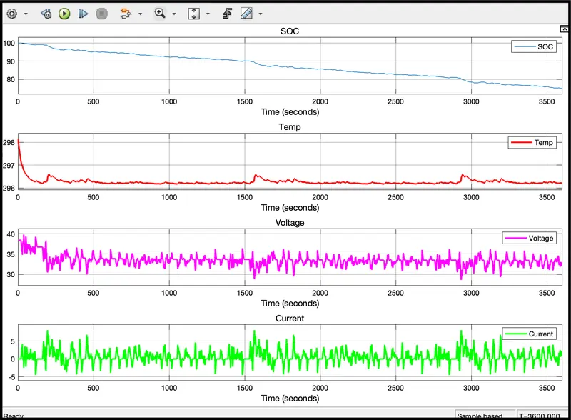
• Here all the values are given to the the blocks and the simulation results are here. Convective area 1m^2 and temperature source23°C(296.15°K)
• The graph is of SOC which is in the decreasing form but in linear, it is some time charging and some time it is discharging as per the current goes positive or negative.it starts from 100% which is full charge after the whole simulation it is at 74.88%.
• The graph is Temperature which is default one I didn't made any changes, so it is decreasing from 298 to 296.2114 which is much good for safety.
• Finally at the last it is voltage fluctuation with respect to time and it starts from 38.4 V and ends at same 32.88 and in between it is increasing and decreasing as the battery is charge or discharge or as per the current drawn or supplied.The max voltage drawn is38.9V and minimum is 29.66V.

Conclusion

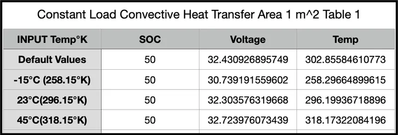
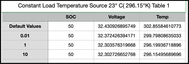
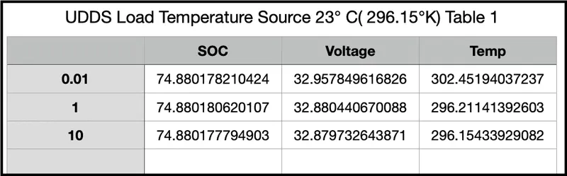
Here both studies for Constant load and UDDS with the simulation of 10 cell series lithium ion battery model and explanation of thermal effects as change in cooling surface at various temperatures using MATLAB had done successfully.The simulation data tabulated from which we can understand at the low temperature the voltage drop much more than high temperature, but SOC has changed slightly.

As surface cooling area is 0.01 M^2 then temp and voltage raised more compare to larger surface area 10 M^2.

The thermal effects and compare life cycle performance at various temperatures, charge & discharge rates using MATLAB.

Simulink -Thermal modelling of battery pack :

Model Explanation :

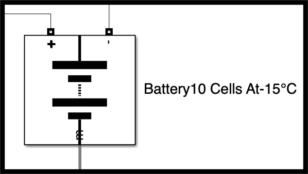
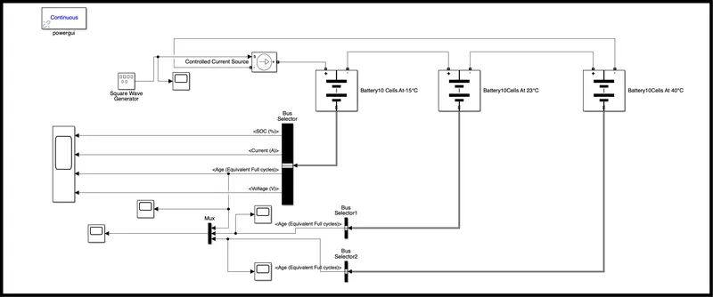
This battery model is found from the directory Electrical/specialised power system/Electric Drives /Extra source. It has two converting ports and one is positive battery terminal and another one is negative battery terminal. And has one output port as named as "m" it gives the multiple vector signal output port giving the SOC ,current, voltage signals, Age, cell temperature etc.

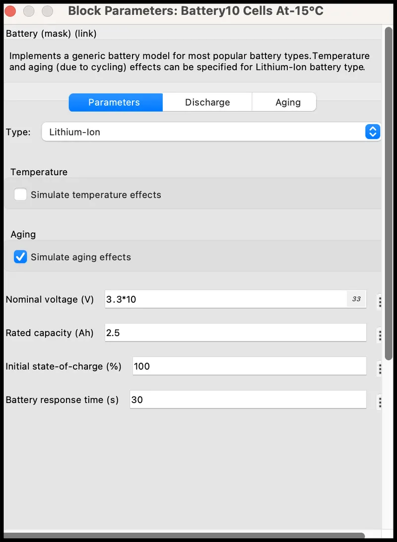
we need to configure the battery as the parameter of 10 series lithium ion battery for that we need to change some parameter in the box as shown in figure. For the 10 series battery the voltage the single cell voltage is add ten times for the series battery. for single cell voltage is 3.3 V. so, for the 10 series cell the voltage will be 33 V.

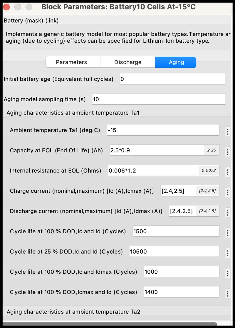
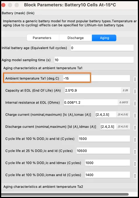
For aging effect in the parameter box we need select the simulate aging effect. After that in that aging already all details are filled as default value from that we need to modify some parameters as shown in figure. Aging sample time is default is very high. But for this simulation we reduce the sample time as 10 sec. And charge and discharge current is default as 0.5C. but we change that to 1C by giving the full current value of 2.5 as shown in below figure.

Square Wave Generator :

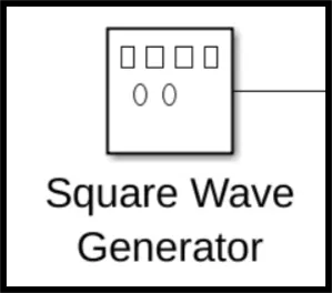
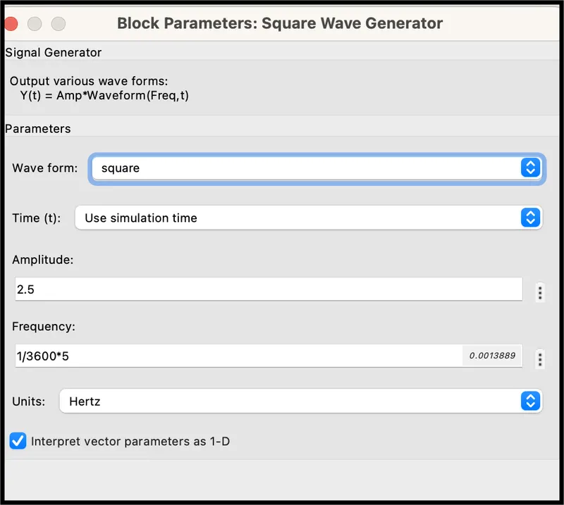
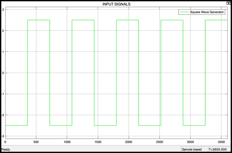
Square wave generator is used for generate the square waves by giving the amplitude and the frequency values in the parameter box.For our simulation we need the full charge and discharge the battery. so for charging at 1C rate which means 2.5 A current we need to charge for 60 min (or) 3600 sec .so we need to give amplitude of 2.5 and for the frequency we need to charge and discharge fully so the time taken is 3600 sec. so the Frequency we set as (1/3600) as shown in below figure.

Bus Selector :

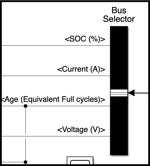
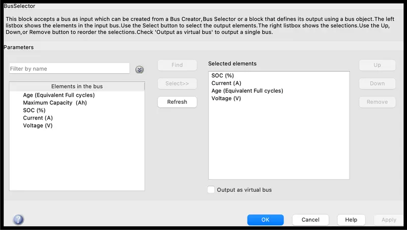
This block accepts a bus as input which can be created from a cell module, Bus selector or a block defines its output using a bus object. The left list box shows the signal in the input bus. Use the select button to select the output signals we need to show. The right list shows the selections. using up and down or remove button to reorder selections as shown in the following figure

Controlled Current source :

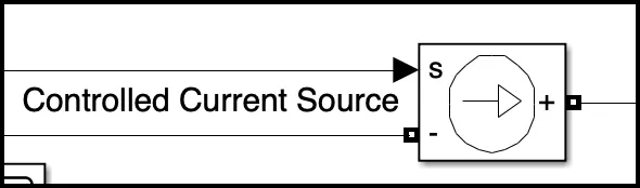
The controlled current source is used for giving the charge and discharge the battery as the controlled source. by connect the battery positive and negative port in current source and the input is the current value given by the wave generator.

In this model the input signals are generated by the wave generator for full charge and discharge the battery. this current is given by the controlled current source to the Battery model. then the battery model output is connected to the bus selector and this selector output is given to scope to view the results.

The run time for this simulation is we need to see the 5 cycles of full charge and discharge of this battery. so we need to run this simulation for 3600*5 times.

Input signals :

Results :

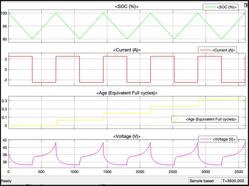
The first plot is shows the SOC in % with the time trace value. We can see the starting the battery has fully charge. As load applied or discharging, it down till 90 % DOD again in charging till 100 %. so the one cycle is one charge and the discharge of the battery. so here we simulate for 5 cycle of the lithium ion battery model.

The Second plot is shows the current level of the battery with the time trace value. Initially battery is fully charged so it is having full 2.5 A current after full load applied it will down 2.5*0.9 =2.25A so in one cycle current in and out from battery.

The third plot is shows the voltage level of the battery with the time trace value. As we see while charging and discharging the voltage level is around 41.2V to 35.16V due to the nominal voltage of this battery is 33V.

Third plot is for Age for equivalent full cycles for the time trace value in this 5 cycles the age value also increase gradually. It around the one complete cycle the age value is 0.06 as shown in the figure so for all 5 cycles the age value is 0.3.

Simulate this model at various temperature :

This simulation we change temperature and observe the result, in the battery parameter box from that Aging parameter we need to change the ambient temperature as -15° C, 23°C and 40°C as shown in the figure.

Result :

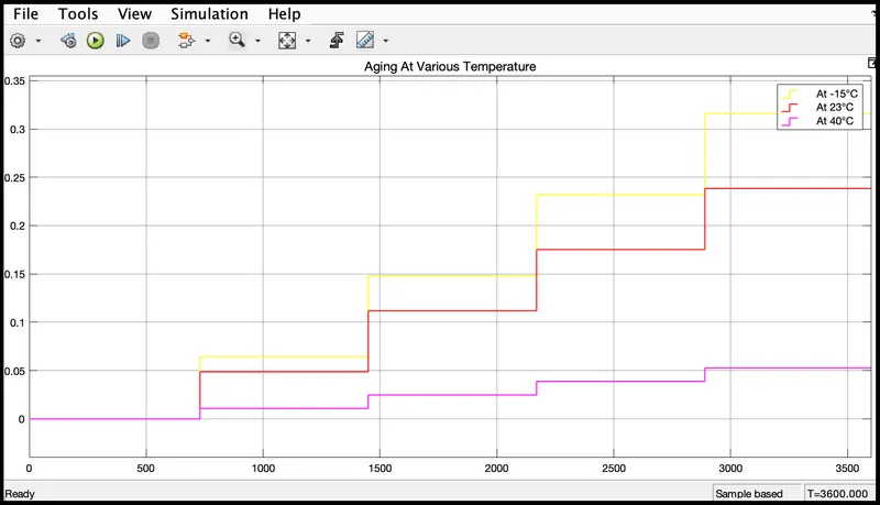
plot is for the Age with the time trace value and the yellow line is for temperature at -15°C. And the red line is for temperature at 23°C. And the magenta line is for temperature at 40°C. so the low temperature(yellow) the aging increase quickly when compared to the 40°C temperature. After 5 cycles the age value is for -15°C(yellow) is 0.315 and 40°C is 0.0528(magenta) so we can understand at the low temperature the aging is faster which means the life cycle will decrease when compare to the high temperatures.

Conclusion

Hence the simulation of 10 cell series lithium ion battery model and explanation of thermal effects and compare life cycle performance at various temperatures using MATLAB is done successfully. from the simulation we can understand at the low temperature the aging is faster which means the life cycle will decrease when compare to the high temperatures.