Project 2 Thermal modeling of battery pack

Output - Default Conditions ( Area of Contact=0.0001 m2 , Temperature Source=298.15 K (25C) )

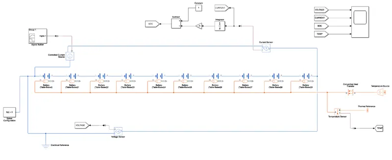
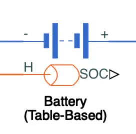
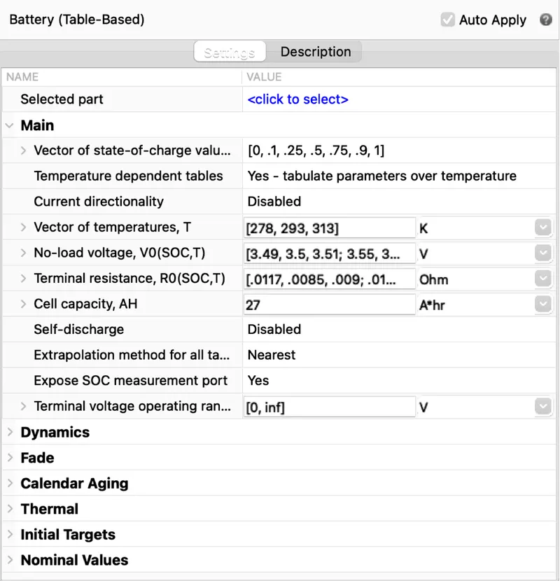
This block models a battery based on tabulated characteristics as functions of state of charge (SOC) and optional temperature (T).

The Battery (Table-Based) block represents a high-fidelity battery model. The block calculates no-load voltage as a function of charge level and optional temperature using lookup tables and includes several modeling options: Self-discharge, Battery fade, Charge dynamics

Default parameters are considered to model the battery

The block represents an ideal current source that is powerful enough to maintain the specified current through it regardless of the voltage across it. The output current is I=Is, where Is is the numerical value presented at the physical signal port

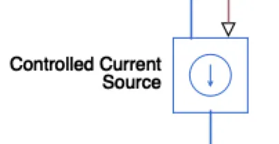
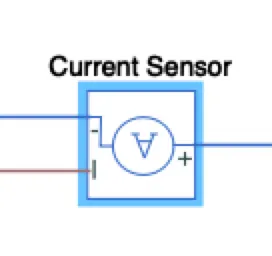
The block represents an ideal current sensor, that is, a device that converts current measured in any electrical branch into a physical signal proportional to the current.

Connections + and - are conserving electrical ports through which the sensor is inserted into the circuit. Connection I is a physical signal port that outputs current value.

Why Sensor?

Sensors - Controls the parameters, Measurement - Just displays the parameters

To some extent, they will have a similar circuit but their end purpose is different so a sensor generates a certain proportional signal which is then processed in a very different cases than in measurement. so current measurement and voltage measurement is just a displays

The block represents an ideal voltage sensor, that is, a device that converts voltage measured between any electrical connections into a physical signal proportional to the voltage.

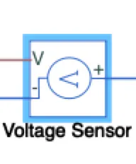
Connections + and - are conserving electrical ports through which the sensor is connected to the circuit. Connection V is a physical signal port that outputs voltage value.

5. Temperature Source -

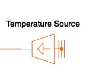
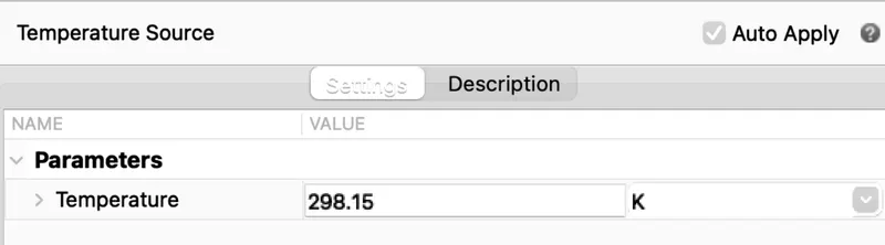
This block represents an ideal energy source in a thermal network that can maintain a constant absolute temperature at the port regardless of the heat flow rate.

6. Temperature Sensor -

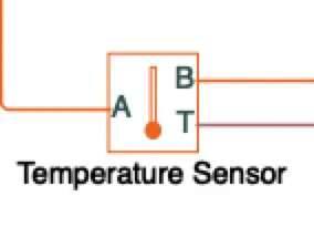
This block measures temperature in a thermal network. There is no heat flow through the sensor. The physical signal port T reports the temperature difference across the sensor. The measurement is positive when the temperature at port A is greater than the temperature at port B.

7. Convective Heat Transfer -

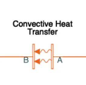
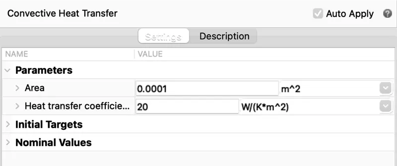
This block models heat transfer in a thermal network by convection due to fluid motion. The rate of heat transfer is proportional to the temperature difference, heat transfer coefficient, and surface area in contact with the fluid.

8. Coulomb Counting Method -

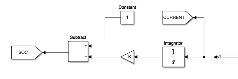
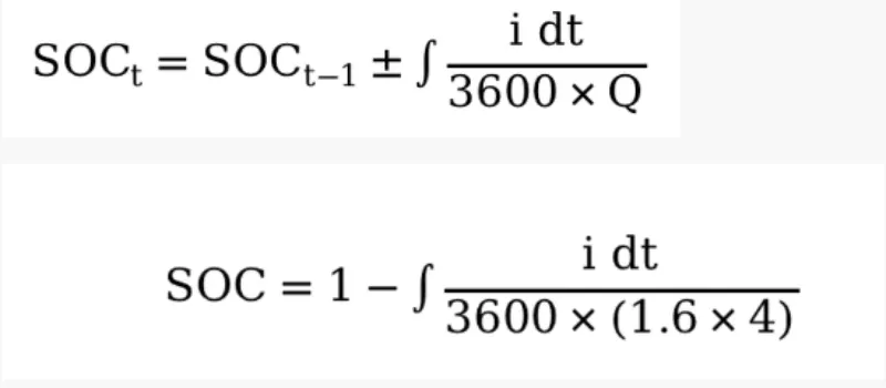
This method is mainly used in the case of module or battery packs SOC estimation

SOC estimation is based on the current integration strategy

Calculates SOC by measuring the current and integrating it in time

9. Signal Builder -

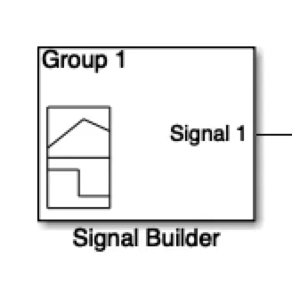
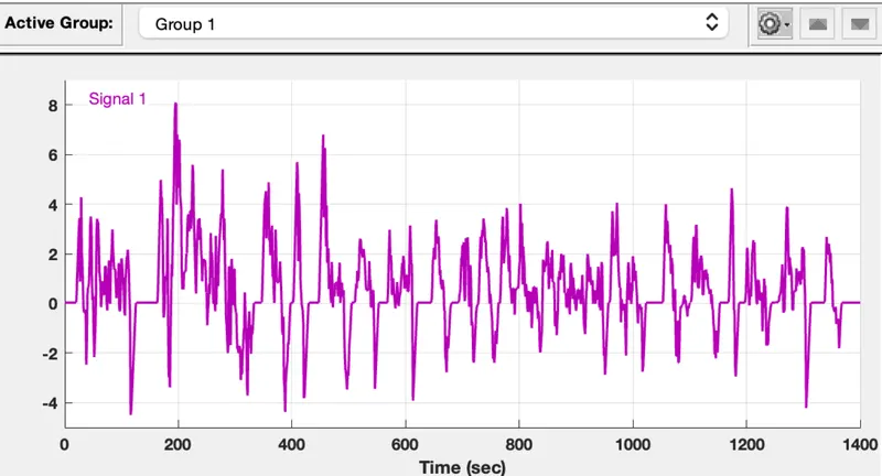
The speed vs time has been converted into Current vs time

The US FTP-72 (Federal Test Procedure) cycle is also called Urban Dynamometer Driving Schedule (UDDS) or LA-4 cycle (CFR 40, 86. App. I) [2656]. This cycle should not be confused with the UDDS schedule for heavy-duty vehicles. The cycle simulates an urban route of 7.5 mi (12.07 km) with frequent stops. The maximum speed is 56.7 mph (91.25 km/h) and the average speed is 19.6 mph (31.5 km/h).

The cycle consists of two phases: (1) 505 s (5.78 km at 41.2 km/h average speed) and (2) 867 s. The first phase begins with a cold start. Weighting factors of 0.43 and 0.57 are applied to the first and second phases, respectively. Emissions are expressed in g/mile or g/km. The same engine driving cycle is known in Australia as the ADR 27 (Australian Design Rules) cycle and in Sweden as A10 or CVS (Constant Volume Sampler) cycle. In Sweden, both phases have the same weighting factors.

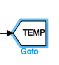
10. Goto Block -

Send signals to From blocks that have the specified tag. If tag visibility is 'scoped', then a Goto Tag Visibility block must be used to define the visibility of the tag. The block icon displays the selected tag name (local tags are enclosed in brackets, [], and scoped tag names are enclosed in braces, {}).

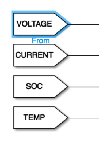
11. From Block -

Receive signals from the Goto block with the specified tag. If the tag is defined as 'scoped' in the Goto block, then a Goto Tag Visibility block must be used to define the visibility of the tag. After 'Update Diagram', the block icon displays the selected tag name (local tags are enclosed in brackets, [], and scoped tag names are enclosed in braces, {}).

Output :

Area of contact - 0.01m2, Temperature Source = 308.15K (35C)

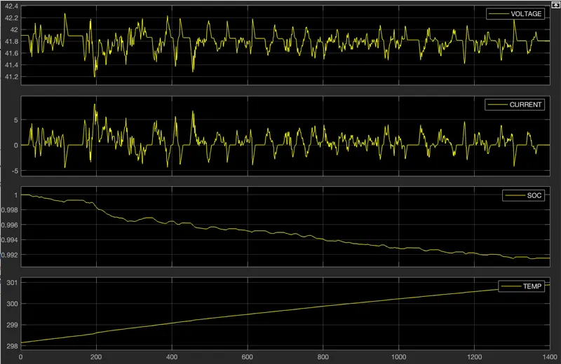
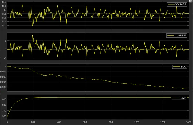
Area of contact - 1m2, Temperature Source = 333.15K (60C)

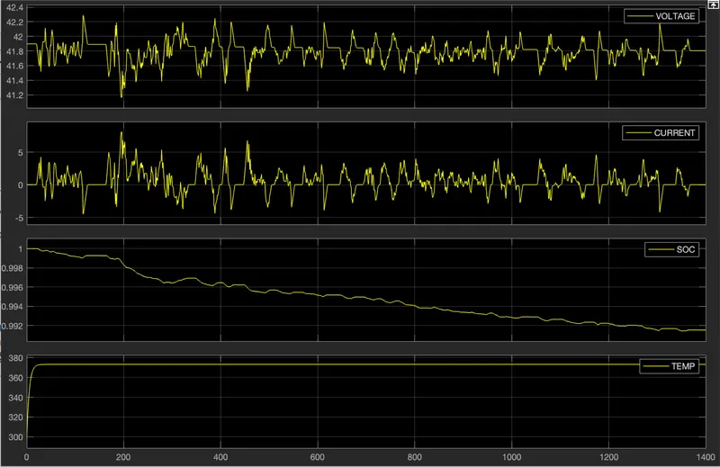
Area of contact - 10m2, Temperature Source = 373.15K (100C)

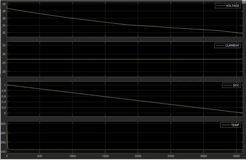
Area of contact - 10m2, Temperature Source = 243.15K (-30C)

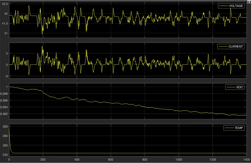
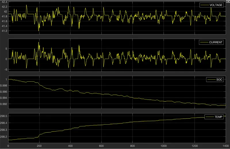
The temperature of the battery pack and the Thermal runaway propagation can be seen in the above graphs which depict that due to the change of point of contact and temperature source the whole battery pack's temperature varies.

The Thermal runaway of the battery Pack can depend on the chemistry and other different parameters with an optimal condition of ( -15C to 40C )

Why the SOC remains constant in all the graphs?

Due to the input Signal builder Block, The dynamics in current vs time graph is so minute and is been charging and discharging continuously

For 1C=27Ah Rate

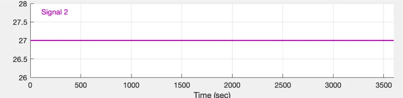
Area of Contact=0.0001 m2 , Temperature Source=298.15 K (25C)

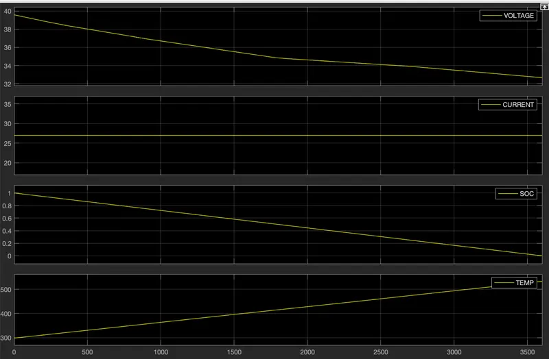
Area of contact - 10m2, Temperature Source = 373.15K (100C)

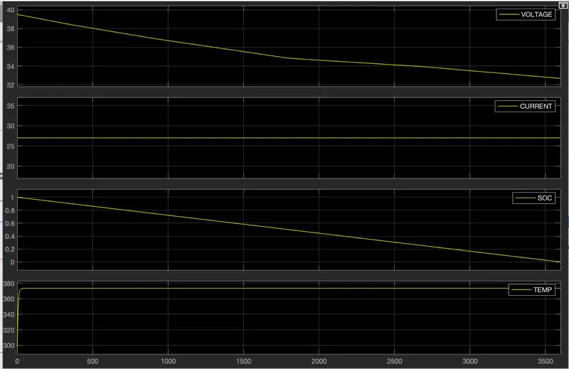
Area of contact - 10m2, Temperature Source = 473.15K (200C)

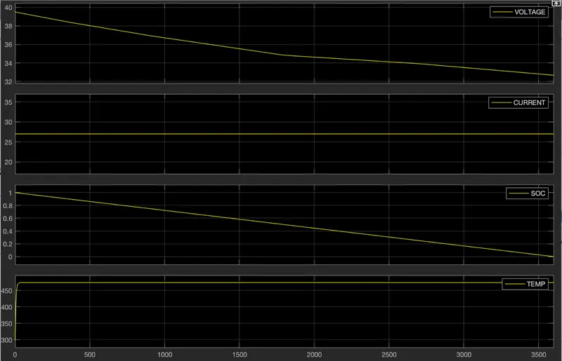
Area of contact - 10m2, Temperature Source = 243.15K (-30C)