Project 2 Thermal modeling of battery pack with different drive cycles

For a 10 cell series lithium ion battery model, simulate the thermal effects and compare life cycle performance at various temperatures, charge & discharge rates using MATLAB ?

To simulate thermal effects we take table based battery cells and connect them in series of 10 cells. We provide different drive cycles and different temperatures to analyse the temperature,SOC changes in the cells and cell series. In order to operate the pack in desired temperatures we will simulate temperature effects.

Simulink Model with Varying Drive Cycle :

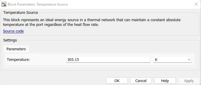
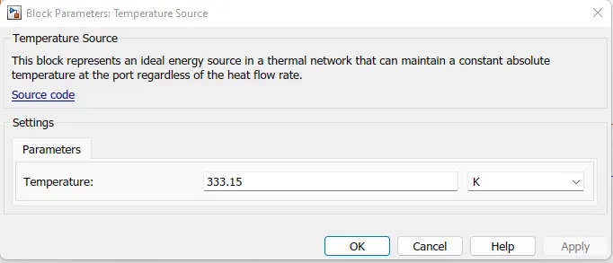
In this model i have taken 10 cells in series with SOC port and given temperature source with different temperature inputs i.e., 303.15K, 313.15K,323.15K,333.15K,343.15K with Convective & Conductive heat transfer areas @ `0.1m^2`,`1m^2` etc.,. I have given varying current signal as input.

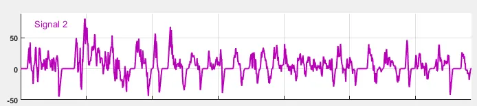
`Figure :` Varying Current Signal

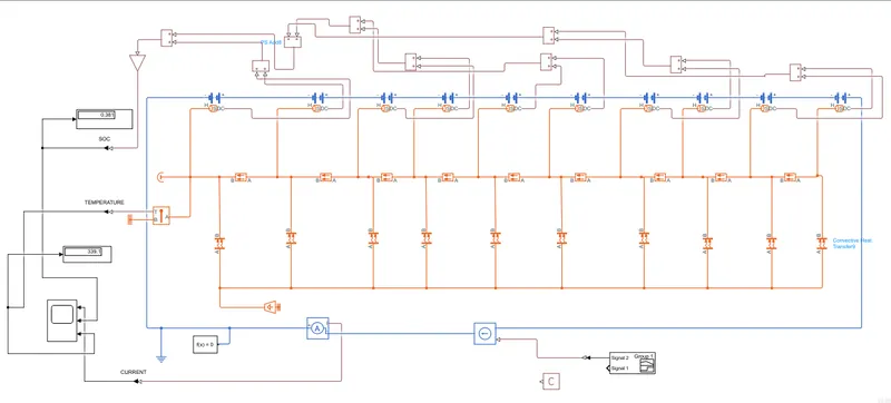
Figure : Simulink Model with varying current signal given from signal builder.

Simulink Model with Constant Current Drive cycle :

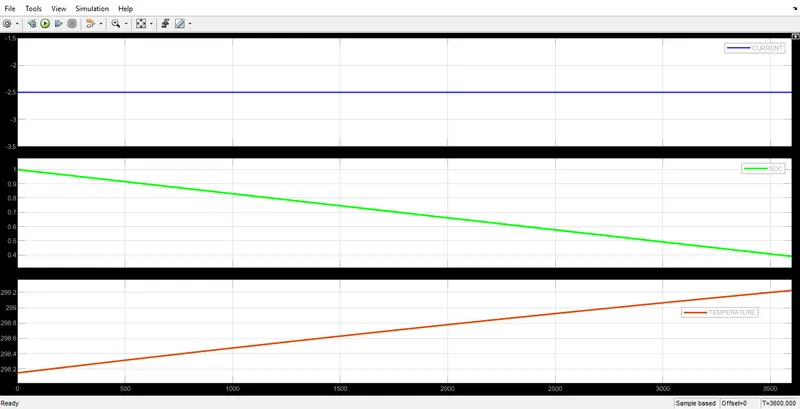
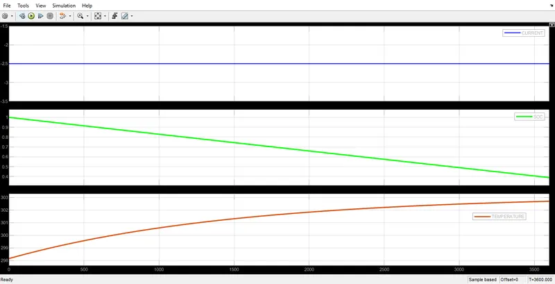
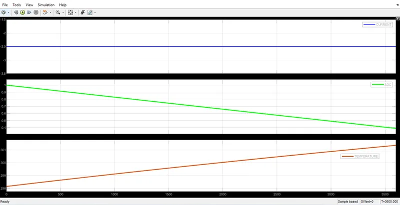
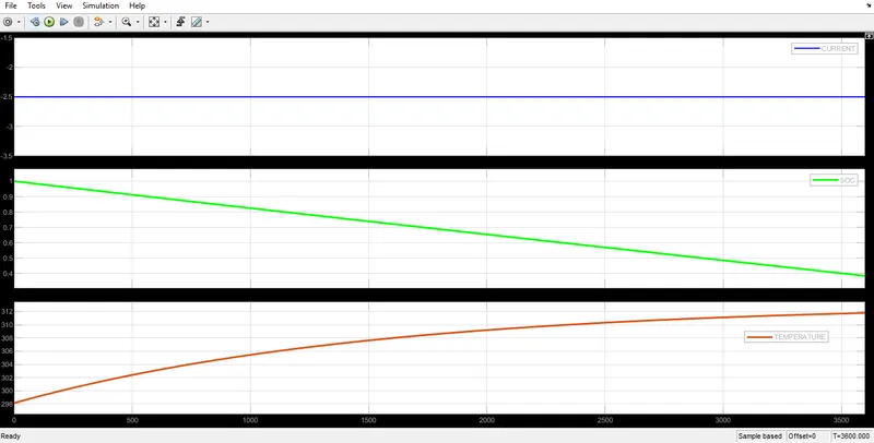
In this model i have taken 10 cells in series with SOC port and given temperature source with different temperature inputs i.e., 303.15K, 313.15K,323.15K,333.15K,343.15K with Convective & Conductive heat transfer areas @ `0.1m^2`,`1m^2` etc.,. I have given constant current signal 2.5A as input.

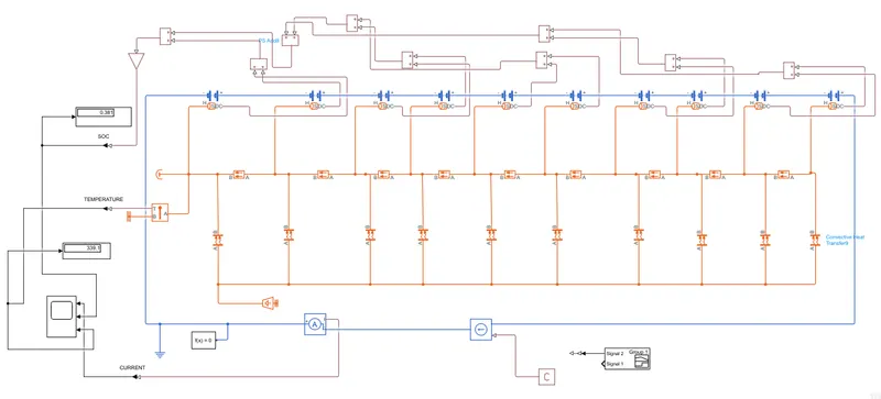
COMPONENTS REQUIRED FOR THE MODEL :

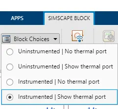
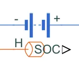
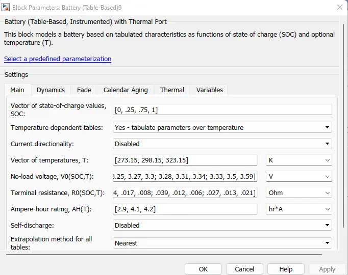
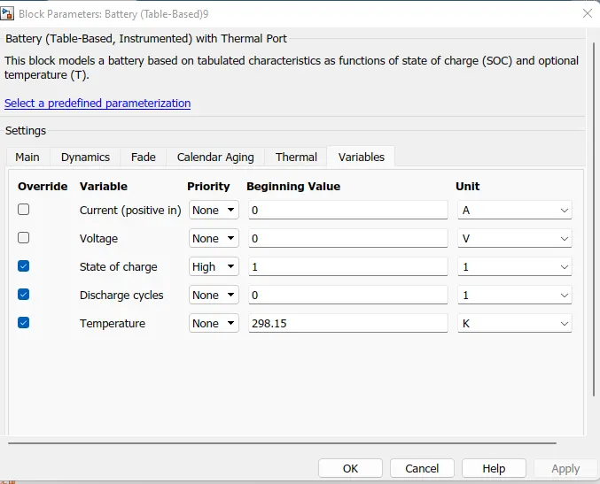
1. Battery (Table-based): I have used table based battery for the simulation. Take a table - based battery and select block choices as "Instrumented Thermal port". Then we get following type of battery with SOC port. The Battery (Table-Based) block represents a high-fidelity battery model. The block calculates no-load voltage as a function of charge level and optional temperature using lookup tables.

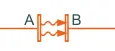
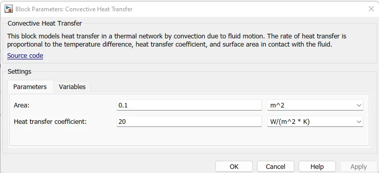
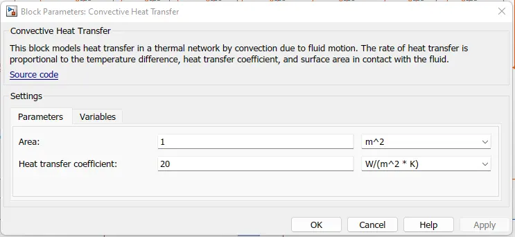
2. Convective Heat Transfer : I have used convective heat transfer to conduct the input source temperature over wide variety of surface areas i.e., 0.1 `m^2` & 1 `m^2`to the battery pack. This block models heat transfer in a thermal network by convection due to fluid motion. The rate of heat transfer is proportional to the temperature difference, heat transfer coefficient, and surface area in contact with the fluid.

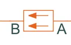
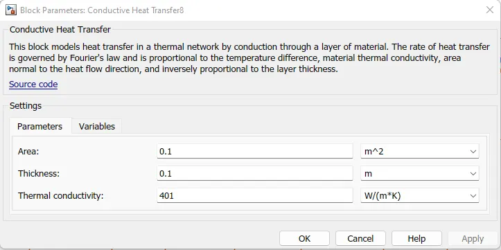
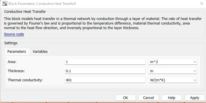
3. Conductive Heat Transfer : I have used conductive heat transfer to transfer heat between cells connected in series with 0.1`m^2` & 1`m^2` surface areas. This block models heat transfer in a thermal network by conduction through a layer of material. The rate of heat transfer is governed by Fourier's law and is proportional to the temperature difference, material thermal conductivity, area normal to the heat flow direction, and inversely proportional to the layer thickness.

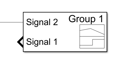
4. Signal Builder : We use this block to build variety of signals. It acts as a signal generator where we can generate custom signal. The Signal Builder block allows you to create interchangeable groups of piecewise linear signal sources and use them in a model. You can quickly switch the signal groups into and out of a model to facilitate testing. In the Signal Builder window, create signals and define the output waveforms.

6. PS Simulink & Simulink PS Convertor : It converts Physical signal to Simulink Signal & Simulink signal to Physical Signal.

7. Display : To display the simulated results we can use this block. We can see the measured value.

5. Electrical Reference : It's electrical ground equivalent used in the simulation.

6. Solver Configuration : It's used to solve equation based math logics.

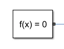
7. Temperature Sensor : It is used to measure temperature in the circuit. This block measures temperature in a thermal network. There is no heat flow through the sensor. The physical signal port T reports the temperature difference across the sensor. The measurement is positive when the temperature at port A is greater than the temperature at port B.

8. Temperature Source : We provide wide variety of temperatures and simulate the mode in varying temperatures environment.This block represents an ideal energy source in a thermal network that can maintain a constant absolute temperature at the port regardless of the heat flow rate.

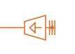
9. Thermal Reference : It is thermal ground which is connected to temperature sensor.It is absolute zero temperature.

10. PS Gain : It is multiply or divide or manipulate the input physical signal value.

11. PS ADD : To add the physical signals.

12. SCOPE : To view the simulated results.

13. Thermal Insulator : It acts as a insulator to thermal conductance. This block represents a terminus in a thermal network with no heat flow and no energy storage. This block is used as an insulation for thermal conserving ports to prevent heat exchange with the environment.

Simulation Results :

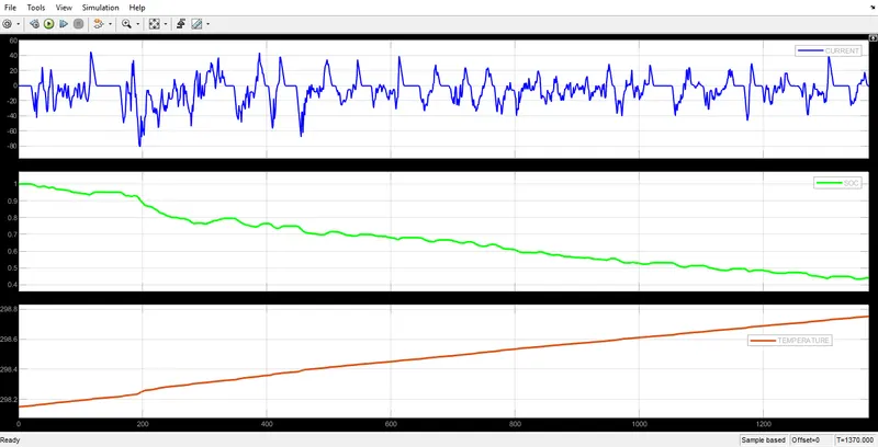
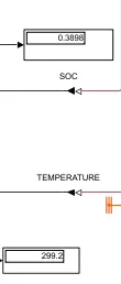
1.For varying drive cycle @ 0.1`m^2` & 1`m^2` heat transfer area :

a. At Temperature = 303.15K or 30 C

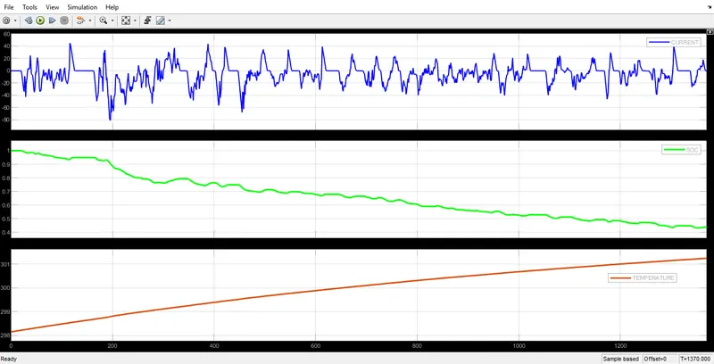
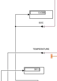
b. At Temperature = 313.15K or 40 C

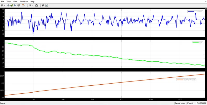
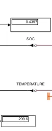
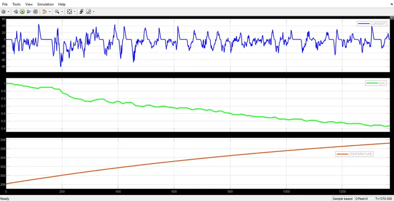
c. At Temperature = 323.15K or 50 C

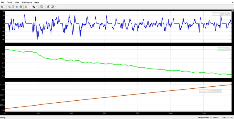
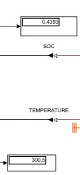
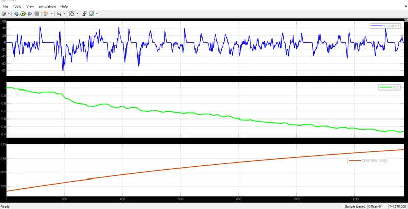
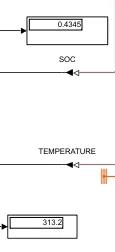
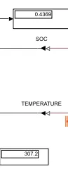
d. At Temperature = 333.15K or 60 C

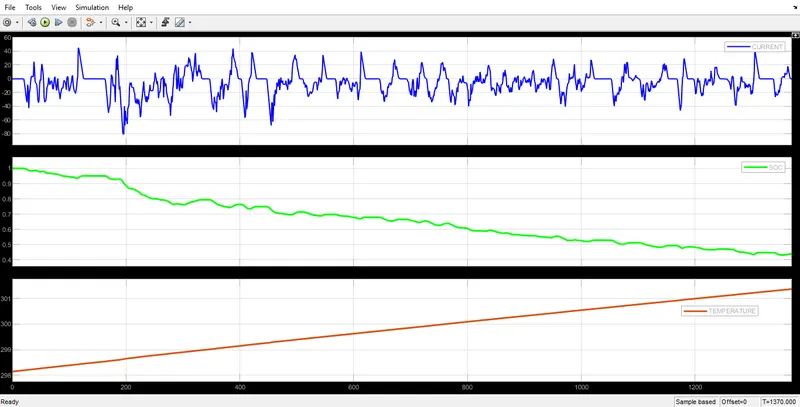
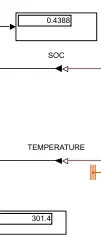
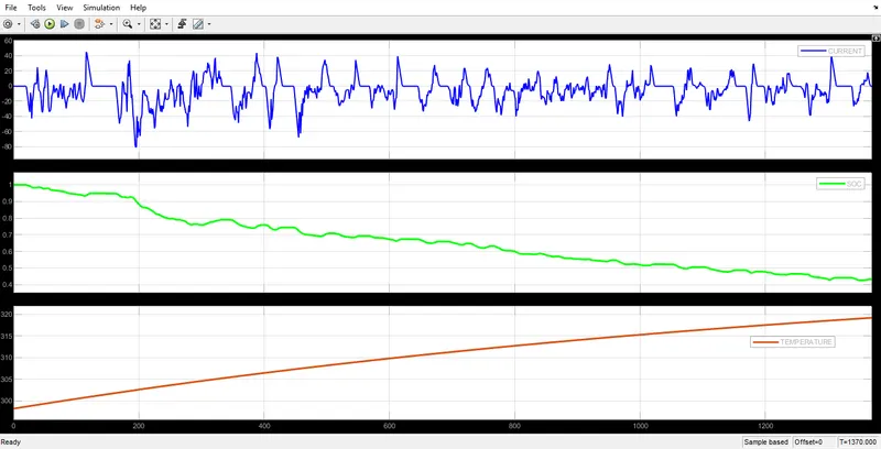
e. At Temperature = 343.15K or 70 C

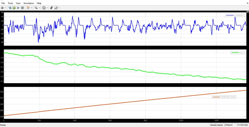
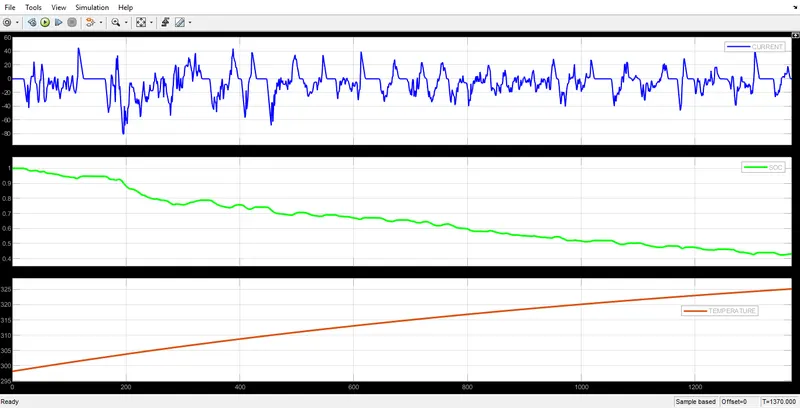
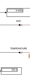
NOTE : As the surface area contact increases the temperature of the pack also increases as we see in above all simulations.

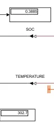
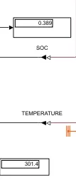
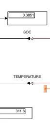
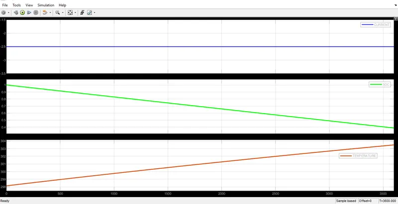
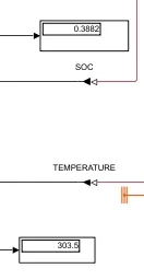
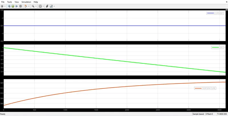
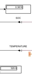
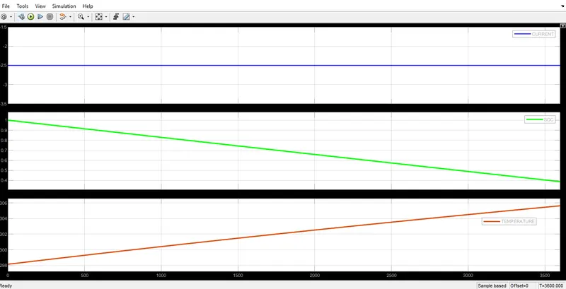
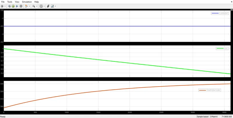
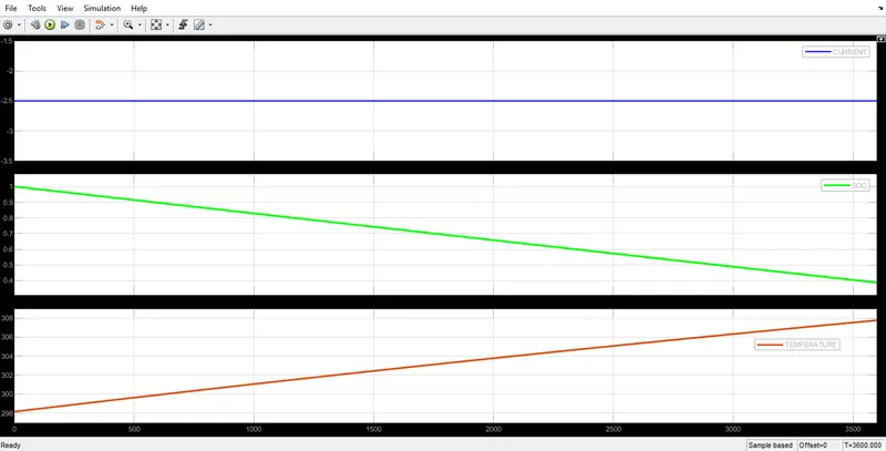
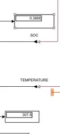
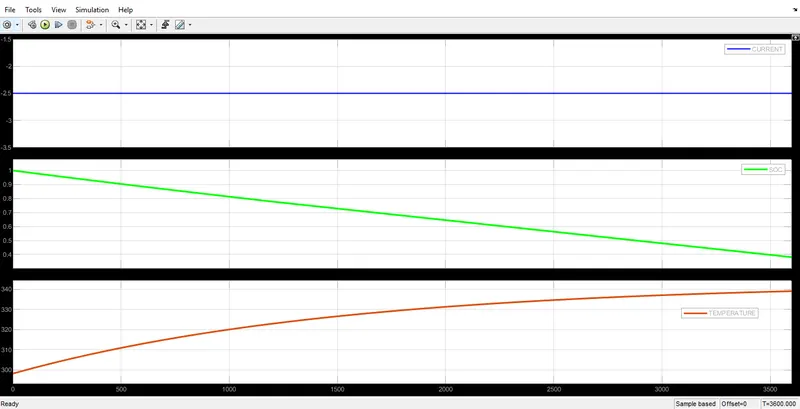
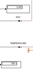
2. For Constant drive cycle @ 0.1`m^2` & 1`m^2` heat transfer area :

a. For Temperature = 303.15 K

b. For Temperature = 313.15 K

c. For Temperature = 323.15 K

d. For Temperature = 333.15 K

e. For Temperature = 343.15 K

For special case of 10 `m^2` heat surface area :

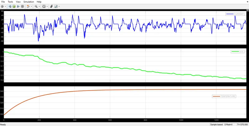
For Varying drive cycle with more heat contact transfer area we can observe that the pack attains input temperature quickly with in 400 sec. So if we run the pack for longer duration at 343.15 K the pack heats up rapidly which might cause thermal failure of the pack. So thermal management techniques should be opted.

Conclusion :

Thus we have simulated the battery pack with different heat surface areas , different temperatures with different drive cycles accordingly. As per my observation when heat surface area through conduction & convection heat transfer takes place with varying surface areas pack takes time to attain input temperatures. Also SOC reduces as per the given drive cycle conditions like for example,

For Varying drive :

At 333.15K or 60 Degrees :

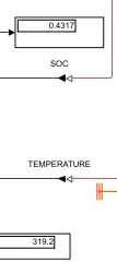
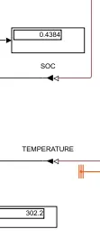
• SOC = 0.438 , Temperature = 301.4 K @ 0.1`m^2` heat surface area;
• SOC = 0.4317 ,Temperature = 319.2 K @ 1`m^2` heat surface area.

Observation : As seen above, SOC reduces when temperature increases (w.r.t surface area of heat addition) .

For Constant drive :

At 333.15K or 60 Degrees :

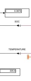
• SOC = 0.387 , Temperature = 305.6 K @ 0.1`m^2` heat surface area;
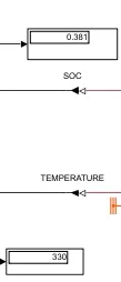
• SOC = 0.387 , Temperature = 305.6 K @ 1`m^2` heat surface area

Observation : As seen above, SOC reduces when temperature increases (w.r.t surface area of heat addition) .

Hence, along with temperature,SOC also varies in above simulations. When Temperature of the pack increases,Slight reduction in SOC is observed in results.