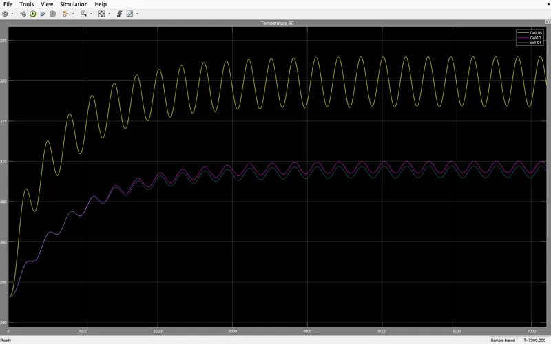
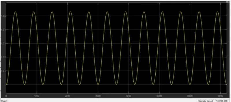
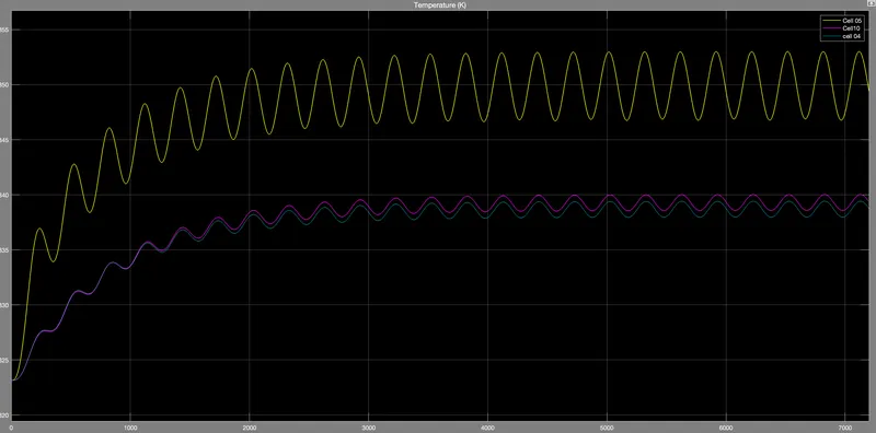
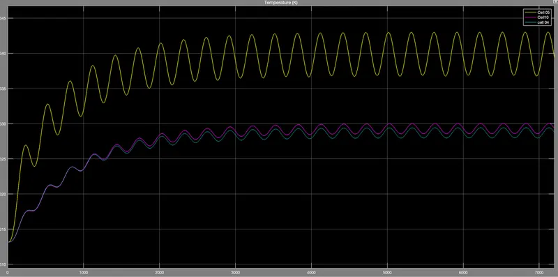
PLOT TEMPERATURE & SOC
try
figure(h1_ssc_lithium_battery_with_fault)
catch
h1_ssc_lithium_battery_with_fault=figure('Name', 'ssc_lithium_battery_with_fault');
end
if ~exist('simlog_ssc_lithium_battery_with_fault','var')
sim('ssc_lithium_battery_with_fault')
end
temp_data = simlog_ssc_lithium_battery_with_fault;
temp_time = temp_data.Cell_01_to_04.Thermal_Model.Battery_Thermal_Mass.T.series.time;
% Extract cell temperature data
temp_T1 = temp_data.Cell_01_to_04.Thermal_Model.Battery_Thermal_Mass.T.series.values;
temp_T2 = temp_data.Cell_5_Fault.Thermal_Model.Battery_Thermal_Mass.T.series.values;
temp_T3 = temp_data.Cell_06_to_10.Thermal_Model.Battery_Thermal_Mass.T.series.values;
% Extract SOC data
temp_SOC1 = temp_data.Cell_01_to_04.Lithium_Cell_1RC.Em_table.SOC.series.values;
temp_SOC2 = temp_data.Cell_5_Fault.Lithium_Cell_1RC.Em_table.SOC.series.values;
temp_SOC3 = temp_data.Cell_06_to_10.Lithium_Cell_1RC.Em_table.SOC.series.values;
ah(1) = subplot(2,1,1);
temp_lh = plot(temp_time/60,[temp_T1 temp_T2 temp_T3],'LineWidth',1);
set(temp_lh(3),'LineStyle','--');
title('Battery Cell Temperature')
ylabel('Temperature (K)')
legend({'Cell 1-4','Cell 5 (Fault)','Cell 06-10'},'Location','SouthEast')
ah(2) = subplot(2,1,2);
temp_lh = plot(temp_time/60,[temp_SOC1 temp_SOC2 temp_SOC3],'LineWidth',1);
set(temp_lh(3),'LineStyle','--');
title('Battery Cell State of Charge')
xlabel('Time (minutes)')
ylabel('State of Charge (0-1)')
legend({'Cell 1-4','Cell 5 (Fault)','Cell 06-10'},'Location','SouthEast')
linkaxes(ah,'x');
% Remove temporary variables
clear temp_data temp_T1 temp_T2 temp_T3 temp_SOC1 temp_SOC2 temp_SOC3 temp_lh ah
MODEL:
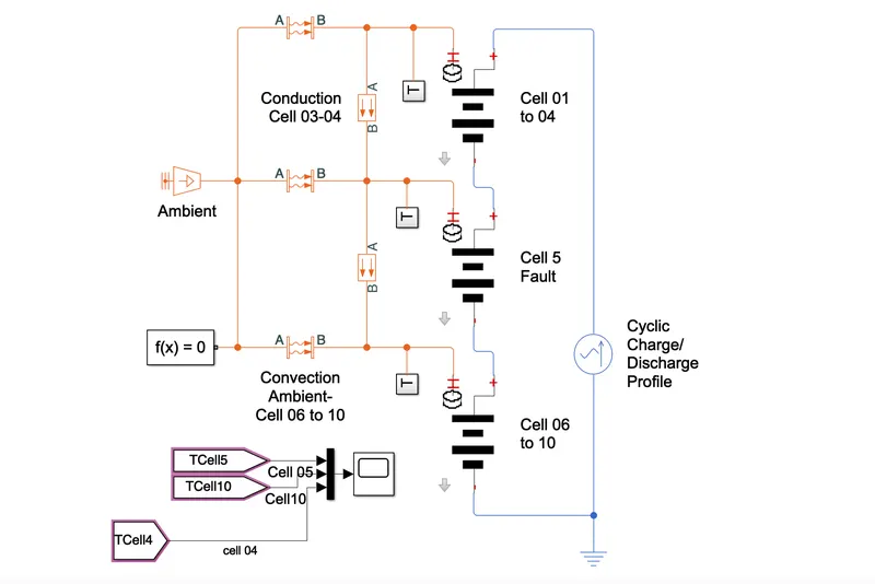
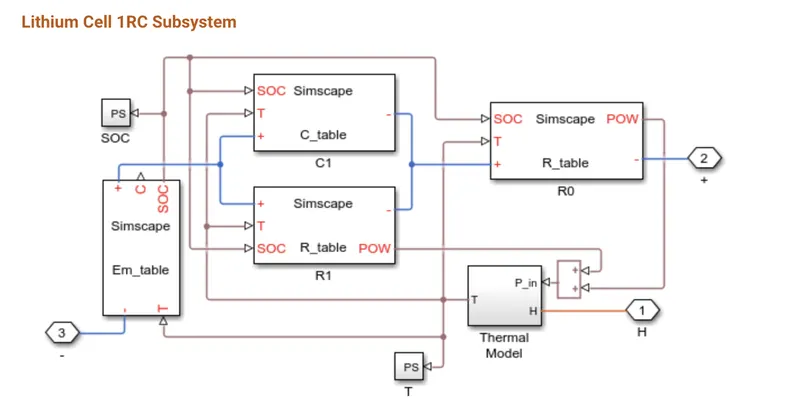
This example shows how to simulate a battery pack consisting of multiple series-connected cells in an efficient manner. It also shows how a fault can be introduced into one of the cells to see the impact on battery performance and cell temperatures. For efficiency, identical series-connected cells are not just simply modeled by connecting cell models in series. Instead a single cell is used, and the terminal voltage scaled up by the number of cells. The fault is represented by changing the parameters for the Cell 10 Fault subsystem, reducing both capacity and open-circuit voltage, and increasing the resistance values.
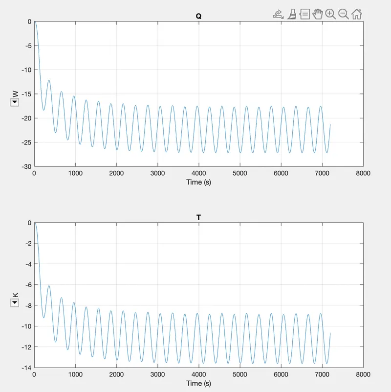
A simple thermal model is used to model battery temperature. It is assumed that cooling is primarily via convection, and that heating is primarily from internal resistance. A battery pack can be modeled by connecting multiple copies of the battery cell block in series.
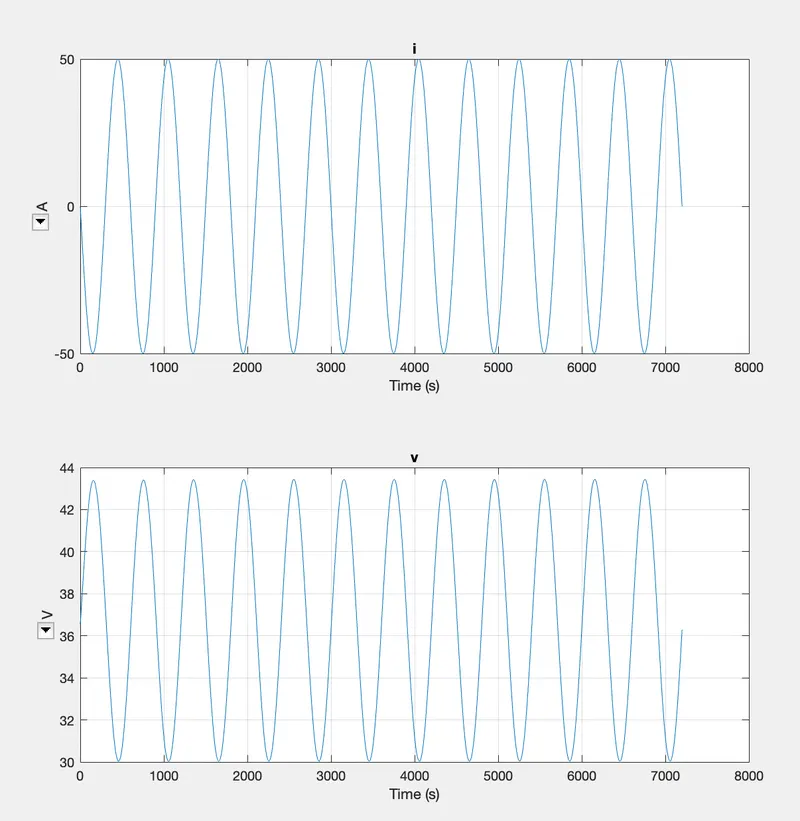
Output:
Ambient
To predict battery performance and to provide SOC estimation in embedded battery management systems. For predicting battery performance, the equivalent circuit of one cell is used as a component in modeling the complete battery pack. The battery pack model is then used inside a larger system-level model that interfaces with other electrical components and transducers, converting electrical energy to mechanical or other physical domains. A typical structure of an equivalent circuit model [1-2, 4, 5, 6, 7, 8, 9] is shown in Figure 1. This circuit contains a voltage source E m , a series resistance R 0 , plus one or more parallel R-C branches connected in series. The model may also contain a parasitic branch, which includes self-discharge and charging losses represented by current I . For lithium electrochemistry, the circuit elements may be modeled using lookup tables for flexibility to match experimental data [4-5]. The parasitic branch (containing Z p and E p ) is often neglected for modeling lithium cells, due to the high coulombic efficiency and low self-discharge under typical operating conditions [4, 6, 9]. To populate the lookup tables, it was necessary to acquire data that exercise each of the parameters in those tables. Pulse type tests such as in Figure 2 provided necessary data about the performance of the battery cell at different points of SOC. Figure 3 below shows a closer look at a single pulse. This pulse provided important information about the open-circuit voltage (OCV) and the circuit dynamics at the given SOC. While collecting these data, other operating conditions such as electrolyte temperature were held as close to constant as possible. The ideal pulse data would have reached steady-state voltage each time before a new pulse begins. However, the settling time was often too slow for practical testing purposes, and we chose a rest time of a few hours. The Figure 4 number shows of just pulses one taken example and dataset. their width To fully had parameterize an effect on the the lookup resolution tables, of the additional data content, datasets since would each be needed pulse provided to cover content the desired at specific operating SOC range breakpoints.
Conduction cell(03-04):
CYCLIC CHARGE/DISCHARGE:
Embedded battery management systems. For predicting battery performance, the equivalent circuit of one cell is used as a component in modeling the complete battery pack. The battery pack model is then used inside a larger system-level model that interfaces with other electrical components and transducers, converting electrical energy to mechanical or other physical domains. A typical structure of an equivalent circuit model [1-2, 4, 5, 6, 7, 8, 9] is shown in Figure 1. This circuit contains a voltage source E m , a series resistance R
293.15K to 20℃:
Thus, capacitor's C1 and C3 in Figure 8 have current I m as an additional lookup table input. We found that, in some pulses, the time constants while polarized under the discharge current would converge to different values from the following recovery phase. Due to the much slower response time of the C2 capacitor, we chose not to provide current dependence that branch since we felt there was not enough data content during the pulse to identify any unique polarization behavior. The Based equivalent on the data circuit in with Figure 4 three containing R-C branches 28 pulses, had eight we variable calculated circuit the corresponding elements that 29 are values a function of SOC of the that operating occurred conditions. before and after These each circuit pulse. elements We represented were represented the values by of lookup each tables. circuit element
CHARGE/DISCHARGE FOR THE LIFE CYCLE:
313.15k to 40℃:
If considering with lookup multiple table versus operating the 29 conditions, points of SOC. these tables would become quite large. In this paper, we considered just one temperature and one discharge current. However, additional independent operating conditions would simply require repeating the estimation process for each condition, and populating additional dimensions of the tables. Based on the data in Figure 4 containing 28 pulses, we calculated the corresponding 29 values of SOC that occurred before and after each pulse. We represented the values of each circuit element with lookup table versus the 29 points of SOC. Because of the three R-C branches and the large number of SOC breakpoints given the data in Figure 4, we had a total of 290 parameters to estimate. We decided it would be unreasonable to attempt a single estimation of all parameters at the same time. We discuss our approach to the problem in the sections that follow.
CHARGE/DISCHARGE FOR THE LIFE CYCLE
323.15K TO 50℃:
One common problem with estimating lookup table parameters was that tables created a large number of additional parameters that increase calculation time; for gradient-based optimizations the algorithm required simulating twice per scalar parameter per iteration of the algorithm. The additional parameters added many more dimensions to the gradient, thus increasing the problem complexity. Because of the above two issues, it was very likely that, assuming a gradient-based optimization algorithm, the error gradient used in the algorithm would have local minima. It was imperative to have good initial conditions and constraints that isolate the effects that each R-C branch had on the model. Additionally, our previous research showed it was extremely important to have data which exercised all parameters in the model [2]. Finally, the size of the data set in Figure 4 was quite large.
CHARGE/DISCHARGE FOR THE LIFE CYCLE
RESULT:
For a 10 cell series lithium ion battery model,simulate the thermal effects and compare life cycle performance at various temperatures, charge & discharge of the We cell, chose including a discharge different test with temperatures uneven and SOC currents. breakpoints, as shown in Figure The discharge test included pulses of different discharge amounts. The high and low SOC pulses were taken while discharging just 1% of cell capacity, and the rest of the data was taken while discharging 10% of cell capacity. This way, we had more data at high and low SOC to better characterize those regions where performance may change dramatically. Figure 4 shows just one example dataset. To fully parameterize the lookup tables, additional datasets would be needed to cover the desired operating range of the cell, including different temperatures and currents. The To determine equivalent the number circuit model of R-C branches with one to R-C use, we branch examined was previously the data during applied the to relaxation a lithium nickel-manganese-cobalt phase. When the pulse current oxide (NMC) was removed, cell [4]. the However, transient lithium response iron was phosphate dictated (LFP) by the cells R 0 exhibit and the R-C more branches complex from dynamics the equivalent including circuit hysteresis. from Figure.
Our research We ignored has shown the that first having sample too after little the or too pulse, much making flexibility the in assumption the model could that the cause instantaneous the optimization voltage to get change stuck. In was this case, described the simulated by the R result 0 parameter. would not We converge then fit at all one toward or more the measured exponential cell equations data. to the data using Curve Fitting Toolbox. Regardless of the number of exponentials we used in this example, they predominantly focused on the slow time constant, as shown in Figure To determine the number of R-C branches to use, we examined the data during the relaxation phase. When the pulse current was removed, the transient response was dictated by the R 0 and the R-C branches from the equivalent circuit from Figure We ignored the first sample after the pulse, making the assumption that the instantaneous voltage change was described by the R 0 parameter. We then fit one or more exponential equations to the data using Curve Fitting Toolbox. Regardless of the number of exponentials we used in this example, they predominantly focused on the slow time constant, as shown in Figure From this result, we determined that having just one or two exponential time constant terms did not produce a satisfactory match to the data. While the curve fit with four exponentials had the lowest residual error, we chose three time constants as a compromise between accuracy and complexity