Project 2 Thermal modeling of battery pack

STUDENT OF ONLINE EV BATCH 16

ANS :

For a 10 cell series lithium ion battery model, simulate the thermal effects and compare life cycle performance at various temperatures, charge & discharge rates using MATLAB.

REQUIRED MODEL :

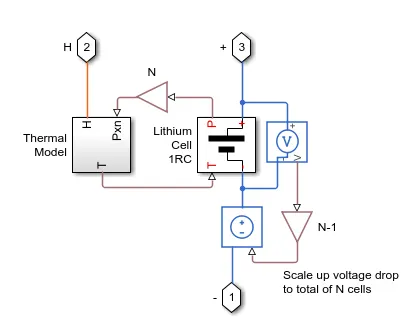
Cell 01 to 04 Subsystem :

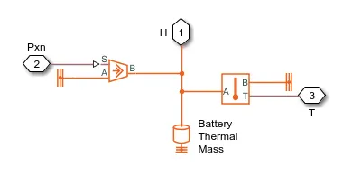
THERMAL MODEL IN SUBSYSTEM :

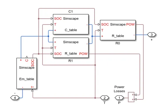
Lithium Cell 1RC Subsystem :

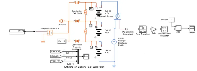
STEPS INVOLVED :

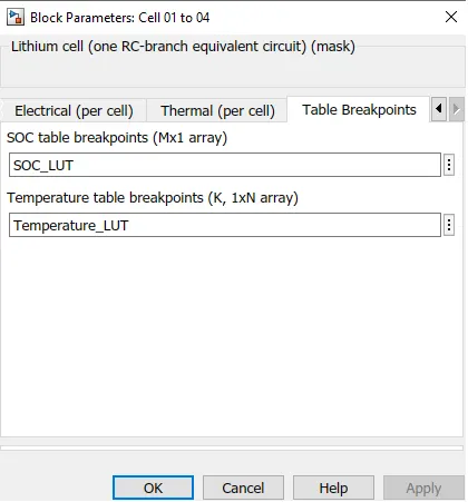
1. CELL1-4 :

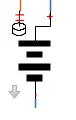
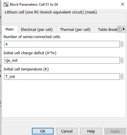
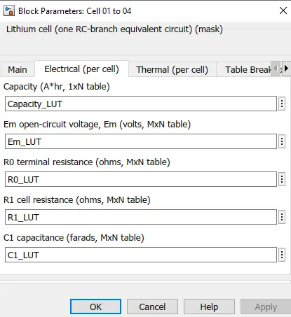
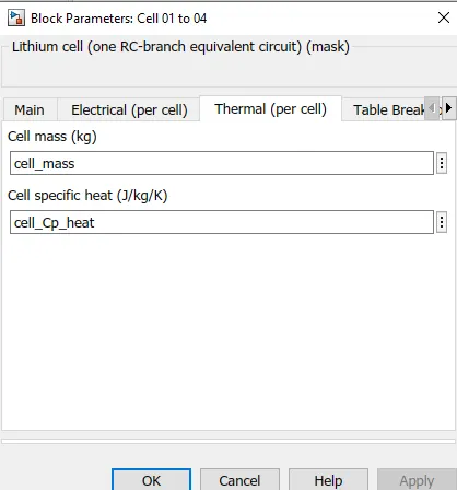
• In this 4 cells are being used in series.

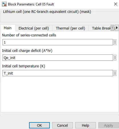
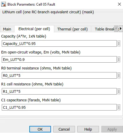
2. CELL 5 :

• There is only one cell in series but in fault condition.

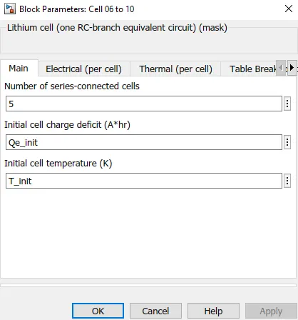
3. CELL 6-10 :

• There is 5 cells in series condition.

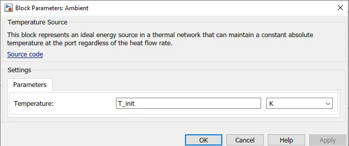
4. TEMPRATURE SOURCE :

• This block represents an ideal energy source in a thermal network that can maintain a constant absolute temperature at the port regardless of the heat flow rate.

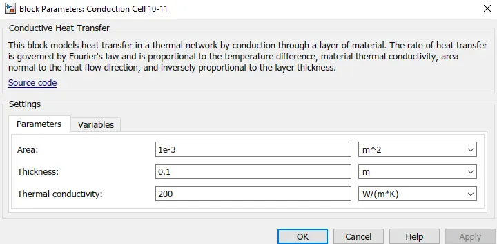
5. CONDUCTIVE HEAT TRANSFER :

• This block models heat transfer in a thermal network by conduction through a layer of material.
• The rate of heat transfer is governed by Fourier's law and is proportional to the temperature difference, material thermal conductivity, area normal to the heat flow direction, and inversely proportional to the layer thickness.

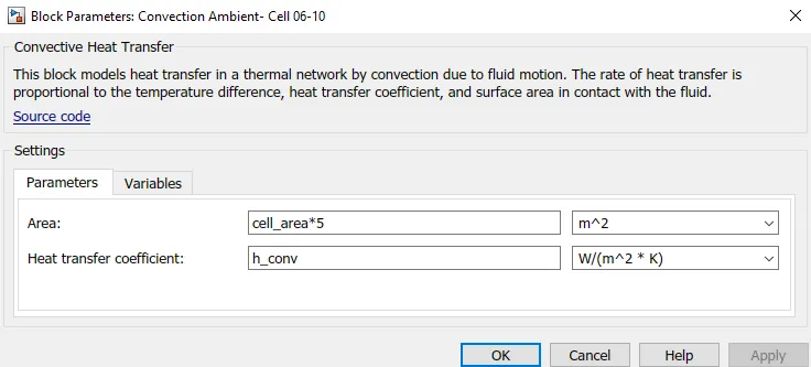
6. CONVECTIVE HEAT TRANSFER :

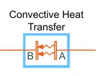
• This block models heat transfer in a thermal network by convection due to fluid motion.
• The rate of heat transfer is proportional to the temperature difference, heat transfer coefficient, and surface area in contact with the fluid

7. TEMPRATURE SENSOR :

• This block measures temperature in a thermal network. There is no heat flow through the sensor.
• The physical signal port T reports the temperature difference across the sensor.
• The measurement is positive when the temperature at port A is greater than the temperature at port B.

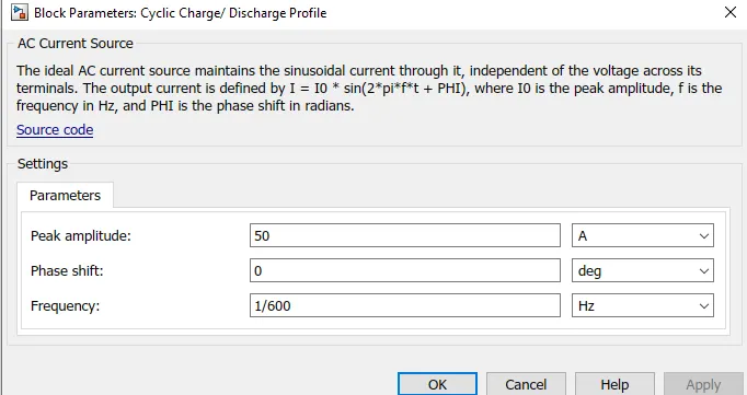
8. CYCLE CHARGE/DISCHARGE PROFILE :

• The ideal AC current source maintains the sinusoidal current through it, independent of the voltage across its terminals.
• The output current is defined by I = I0 * sin(2*pi*f*t + PHI), where I0 is the peak amplitude, f is the frequency in Hz, and PHI is the phase shift in radians.

9. SOC CALCULATION :

For SOC calculation we have designed a mathematical model as below :

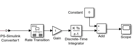
Current sensor output has been given to PS-Simulink convertor then it passes through the rate transition and then through the gain block and integrated in discrete form then given to add block and a constant having value 0 is provided to get the below graph.

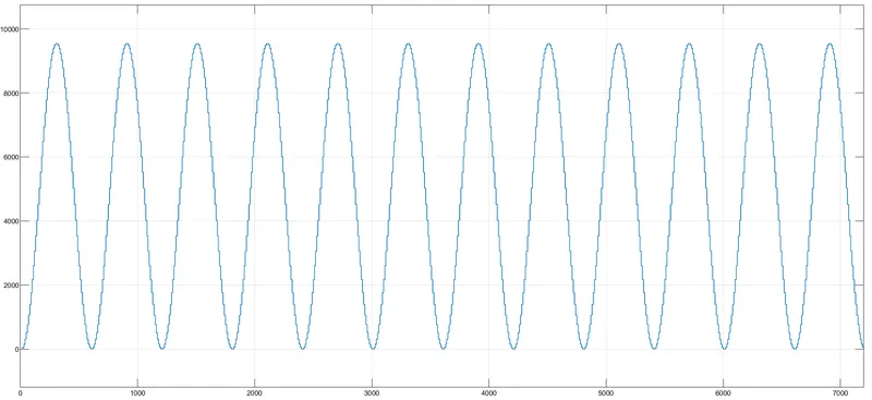
For Ist 300s our SOC reaches to 95% during charging then fro 300s for discharging with the same value. In 1 h, it has completed the 6 complete cycles with charging and discharging.

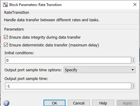
10. RATE TRANSITION :

• Handle data transfer between different rates and tasks.

11. GAIN BLOCK :

• Element-wise gain (y = K.*u) or matrix gain (y = K*u or y = u*K).

12. DISCRETE-TIME INTEGRATOR :

• Discrete-time integration or accumulation of the input signal.

13. ADD BLOCK :

• Add or subtract inputs. Specify one of the following:

a) character vector containing + or - for each input port, | for spacer between ports (e.g. ++|-|++)

b) scalar, >= 1, specifies the number of input ports to be summed.

When there is only one input port, add or subtract elements over all dimensions or one specified dimension

SIMULATION RESULT :

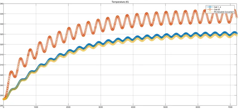
Here, we can observe the graph of all cells connected in series. Where, Cell1_4 and Cell6_10 has lower value of temprature which is 317K to 325K. And the faulty cell5 has the temprature as 312K to 334K.

SOC CURVE :

As per model, Current sensor output has been given to PS-Simulink convertor then it passes through the rate transition and then through the gain block and integrated in discrete form then given to add block and a constant having value 0 is provided to get the below graph.

For Ist 300s our SOC reaches to 95% during charging then fro 300s for discharging with the same value. In 1 h, it has completed the 6 complete cycles with charging and discharging.

MATLAB HELP MODEL :

Lithium-Ion Battery Pack With Fault For 20 Cells :

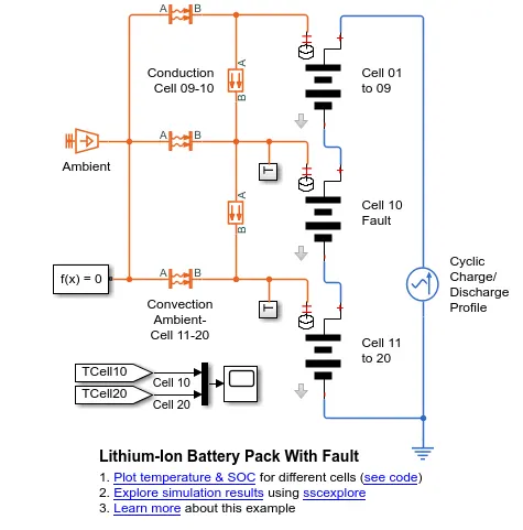
• This example shows how to simulate a battery pack consisting of multiple series-connected cells in an efficient manner.
• It also shows how a fault can be introduced into one of the cells to see the impact on battery performance and cell temperatures.
• For efficiency, identical series-connected cells are not just simply modeled by connecting cell models in series.
• Instead a single cell is used, and the terminal voltage scaled up by the number of cells.
• The fault is represented by changing the parameters for the Cell 10 Fault subsystem, reducing both capacity and open-circuit voltage, and increasing the resistance values.

MATLAB SCRIPT FOR 20 CELLS :

% Plotting script for example battery model ssc_lithium_battery_with_fault.
% This example shows how to model a series of lithium-ion cells where one
% of the cells develops a fault. The data used for each cell is the same
% as for the ssc_lithium_cell_1RC example model, and is based on T. Huria,
% M. Ceraolo, J. Gazzarri, R. Jackey. "High Fidelity Electrical Model with
% Thermal Dependence for Characterization and Simulation of High Power
% Lithium Battery Cells," IEEE International Electric Vehicle Conference,
% March 2012.

% Copyright 2014 The MathWorks, Inc.

try
figure(h1_ssc_lithium_battery_with_fault)
catch
h1_ssc_lithium_battery_with_fault=figure('Name', 'ssc_lithium_battery_with_fault');
end

if ~exist('simlog_ssc_lithium_battery_with_fault','var')
sim('ssc_lithium_battery_with_fault')
end
temp_data = simlog_ssc_lithium_battery_with_fault;
temp_time = temp_data.Cell_01_to_09.Thermal_Model.Battery_Thermal_Mass.T.series.time;

% Extract cell temperature data
temp_T1 = temp_data.Cell_01_to_09.Thermal_Model.Battery_Thermal_Mass.T.series.values;
temp_T2 = temp_data.Cell_10_Fault.Thermal_Model.Battery_Thermal_Mass.T.series.values;
temp_T3 = temp_data.Cell_11_to_20.Thermal_Model.Battery_Thermal_Mass.T.series.values;

% Extract SOC data
temp_SOC1 = temp_data.Cell_01_to_09.Lithium_Cell_1RC.Em_table.SOC.series.values;
temp_SOC2 = temp_data.Cell_10_Fault.Lithium_Cell_1RC.Em_table.SOC.series.values;
temp_SOC3 = temp_data.Cell_11_to_20.Lithium_Cell_1RC.Em_table.SOC.series.values;

ah(1) = subplot(2,1,1);
temp_lh = plot(temp_time/60,[temp_T1 temp_T2 temp_T3],'LineWidth',1);
set(temp_lh(3),'LineStyle','--');
title('Battery Cell Temperature')
ylabel('Temperature (K)')
legend({'Cell 1-9','Cell 10 (Fault)','Cell 11-20'},'Location','SouthEast')
ah(2) = subplot(2,1,2);
temp_lh = plot(temp_time/60,[temp_SOC1 temp_SOC2 temp_SOC3],'LineWidth',1);
set(temp_lh(3),'LineStyle','--');
title('Battery Cell State of Charge')
xlabel('Time (minutes)')
ylabel('State of Charge (0-1)')
legend({'Cell 1-9','Cell 10 (Fault)','Cell 11-20'},'Location','SouthEast')

linkaxes(ah,'x');

% Remove temporary variables
clear temp_data temp_T1 temp_T2 temp_T3 temp_SOC1 temp_SOC2 temp_SOC3 temp_lh ah

SCRIPT RESULT :

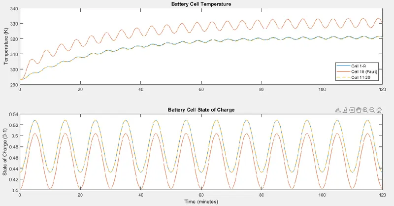
Here, we can observe the graph of all cells connected in series. Where, Cell1_9 and Cell11_20 has lower value of temprature which is 317K to 325K. And the faulty cell5 has the temprature as 312K to 334K.

For Ist 300s our SOC reaches to 95% during charging then fro 300s for discharging with the same value. In 1h, it has completed the 6 complete cycles with charging and discharging.