Project 2 Thermal modeling of battery pack
For a 10 cell series lithium ion battery model, simulate the thermal effects and compare life cycle performance at various temperatures, charge & discharge rates using MATLAB.
Lithium-ion batteries (LIBs) are widely used in electric vehicles (EVs), grid-tied stationary energy storage systems, and several other consumer electronics primarily dueto their high voltage rating (>4 V/cell) and high energy density (~265 (W h) L−1) andlonger operational life. The use of LIBs in automotive and aerospace applications has led to larger cell sizes and large battery packs for a higher driving range and the requirement for more aggressive charging and discharging. However, thermal instability and temperaturedependent nonlinear behavior is some of the common concerns behind the safe and reliable operation of LIB systems. It is noticed that the operation of batteries outside the safe operating temperature directly affects the performance of LIBs, such as cycle life, efficiency, reliability and safety. Researchers investigating the thermal performance of LIB showed that the best operating temperature range is from 25 ◦C to 40 ◦C [1,2]. Richardson et al. [3] demonstrated that the difference between the core and surface temperature could reach more than 10 ◦C during real-life applications, especially during the high discharging condition and fluctuating load current demand. The excessive temperature difference and the
accumulation of a large amount of heat inside the cell could lead to thermal runaway or even explosions and fire [4]. That necessitates the employment of a battery management system (BMS) for effective monitoring of battery parameters (current, voltage, temperature), estimation of battery states (state of charge (SOC), state of health (SOH), remaining useful
life (RUL), state of temperature (SOT) [5]). Research studies demonstrated that SOC [6], SOH [7], and remaining storage capacity [8] are a function of temperature; thus, the estimation of the battery states also depends on the accurate estimation of cell temperature.
The Columbic efficiency of a cell is greatly affected by the cell temperature during the charging and discharging period. Few other popular functionalities of BMS include cell balancing [9] and fault detection/diagnosis [10] to ensure optimum capacity utilization, operational safety, reliability, and longer battery life often requires temperature information of an individual cell and battery pack as well. Therefore, accurate information of core and surface temperature is highly crucial for effective thermal management and safety of a LIB pack. Moreover, in cold climate areas, the battery capacity is drastically reduced due
to low-temperature operation that requires preheating the battery to a suitable range for optimum performance [11,12]. It is also evidenced that for every 0.1 ◦C beyond the safe operating region the battery capacity degrades by about 5% [13]. It is evidenced that maximum heat is generated during the discharging period especially with fast discharging [14]. Therefore, accurate temperature estimation is essential for effective thermal management and safety during fast charging and discharging and preheating of the cell to minimize
capacity fade.
In summary, it could be stated that the accurate information of cell temperature is undoubtedly serving as the essential basis for the thermal management and safety of LIB. While the surface temperature of each cell can be measured by installing a temperature sensor on each cell, the core or internal temperature measurement directly using physical sensors is challenging. Moreover, installing a temperature sensor on each cell surface is not practically feasible from a system cost, space and weight point of view as any high-capacity battery pack used in EVs and grid-tied systems essentially consists of thousands of individual cells. Researchers have also incorporated multi-dimensional sensing and self-healing functions into a single battery cell to develop a smart battery [15–18]. Smart cells are typically capable of parameter measurements and estimation of cell states including the state of temperature. Despite the modularized application of BMS in smart batteries, accurate
temperature estimation is still required, as otherwise installing sensors in each cell results in high implementation cost and complexity. Therefore, researchers are struggling hard to develop a high-fidelity, accurate, easy-to-implement, and computationally inexpensive online temperature estimation strategy suitable for low-cost onboard BMS. Several temperature estimation techniques have been proposed by researchers so far. Each different type of method has its advantages and limitations with respect to the above-mentioned features of an optimum BMS. Therefore, a summary of all the prominent techniques would be very helpful to researchers and developers serving as a baseline for further research and as a guideline for selecting appropriate techniques suitable for a specific requirement. However, such a summary with detailed discussion on current progress and explanation of the existing issues, challenges and future research scopes has not yet been presented in the literature. Therefore, this article covered the research gap by conducting a comprehensive review of the state-of-the-art temperature estimation strategies reported in the literatureso far.
The paper is organized as follows: In Section 2, generic temperature estimation strategy of LIB is presented. The classification of temperature estimation strategies is presentedin Section 3. Section 4 is dedicated to presenting the existing estimation techniques, their evolutions, limitations and challenges. It should be noted that temperature estimation strategies for LIBs reported in the literature between 2010 to 2021 are primarily considered. However, few prominent research articles published between 1990 to 2010 are also considered for understanding the fundamentals and evolution of temperature estimation
Energies 2021, 14, 5960 3 of 25 schemes. Commonly used search platforms, such as “Google Scholar”, “Science Direct”,
and IEEE Xplore, were used to find research articles published within this tenure. The search criteria were “Temperature Estimation of Lithium-ion Batteries”. Section 5 discusses the current issues, challenges and future research recommendations. Finally, Section 6 is dedicated to a summary of the major findings and concluding remarks.
2. Generic Temperature Estimation Strategy
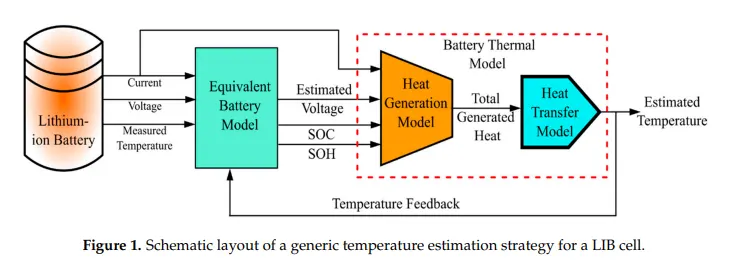
Irrespective of battery chemistry, heat is accumulated inside the battery during the charging/discharging even during idle conditions, majorly due to several largely exothermic chemical and electrochemical reactions as well as transport processes. If the heat transfer from the battery to the surroundings is not sufficient, then the heat gets accumulated inside the battery resulting in an increase in core and surface temperature, thereby risking thermal runaway. This phenomenon is even more prominent in the case of hard-cased insulated batteries (as used in EVs), under fast charging/discharging and the operation in hot environments. Heat dissipation is worse in cylindrical LIBs that are extensively used in high-capacity LIB packs. Therefore, a typical temperature estimation scheme consists of two models, namely, a heat generation model and a heat transfer model [19]. Often, a battery electrical model is also used to estimate the total heat generation using Bernardi’s [20] heat generation model whereas few other models use a mathematical form of battery electrochemistry to calculate the heat generation. Adaptive estimation strategies also consider the influence of different battery states, such as SOC and SOH, as the battery temperature is a function of these battery states. Then, the heat transfer model takes the estimated total heat quantity as well as few other external measurements such as ambient temperature to predict the temperature of that cell. Closed-loop estimation schemes use the measured or the estimation temperature as feedback to improve the prediction accuracy. A
schematic layout of a generic temperature estimation strategy for LIB is shown in Figure 1.
Classification of Temperature Estimation Strategies
As shown in Figure 1, typically, a temperature estimation scheme consists of a heat generation model and a heat transfer model. The heat generation models reported in the literature can be broadly classified from two different aspects; based on modelling strategy and based on the source of heat generation. Heat generation models based on modelling strategy can be classified into three groups, physics-based electrochemical models [21–24], equivalent circuit models (ECM) [25–27], black-box models [28–30]. In contrast, based on the source of heat generation, these models can be grouped as a concentrated model, distributed model [31] and heterogeneous model [25,32]. The concentrated heat generation model considers that all heat is generated at the core only, usually considered to reduce the modelling complexity. The distributed heat generation
Figure 1. Schematic layout of a generic temperature estimation strategy for a LIB cell. 3. Classification of Temperature Estimation Strategies As shown in Figure 1, typically, a temperature estimation scheme consists of a heat generation model and a heat transfer model. The heat generation models reported in the literature can be broadly classified from two different aspects; based on modelling strategy and based on the source of heat generation. Heat generation models based on modelling
strategy can be classified into three groups, physics-based electrochemical models [21–24], equivalent circuit models (ECM) [25–27], black-box models [28–30]. In contrast, based on the source of heat generation, these models can be grouped as a concentrated model, distributed model [31] and heterogeneous model [25,32]. The concentrated heat generation model considers that all heat is generated at the core only, usually considered to reduce the modelling complexity. The distributed heat generation model considers that uniform heat is generated throughout the entire cell geometry whereas the heterogeneous model can capture different heat generation from difference cell layers usually resulting in temperature
and current density gradients inside the cell. The heterogeneous models are more detailed thus can produce highly accurate predictions; however, these are most complex and requireEnergies 2021, 14, 5960 4 of 25 extensive experiments for modelling. Distributed heat generation models are a balance between the concentrated and heterogeneous models. The heat transfer models can be classified into finite element analysis (FEA)-based models [27,33–36], heat capacitor-resistor
models (lumped or distributed parameter) [28,37–40], and data-driven techniques. Heat capacitor–resistor-based models use the analogy between electrical and thermal systems.
A heat capacitor–resistor can be further classified as mentioned in Figure 2. Lumped parameter models are simple and useful for online applications, however, only one or two average temperatures can be predicted with these models whilst the battery temperature distribution is not spatially uniform, especially in larger capacity cylindrical LIB cells. On the other hand, complex distributed models [41,42] can describe the detailed temperature distribution in a cell, however, they are not suitable for online application due to their computational complexity. Several other detailed models of LIB accounting for the thermal
characteristics of different layers are studied in [43–48]. A two-state/node model provides information on core and surface temperature whereas a one-state/node model can provide only core temperature. model considers that uniform heat is generated throughout the entire cell geometry whereas the heterogeneous model can capture different heat generation from difference cell layers usually resulting in temperature and current density gradients inside the cell. The heterogeneous models are more detailed thus can produce highly accurate predictions; however, these are most complex and require extensive experiments for modelling. Distributed heat generation models are a balance between the concentrated and heterogeneous models. The heat transfer models can be classified into finite element analysis (FEA)-based models [27,33–36], heat capacitor-resistor models (lumped or distributed parameter) [28,37–40], and data-driven techniques. Heat capacitor–resistor-based models use the analogy between electrical and thermal systems. A heat capacitor–resistor can be further classified as mentioned in Figure 2. Lumped parameter models are simple and useful for online applications, however, only one or two average temperatures can be predicted with these models whilst the battery temperature distribution is not spatially uniform, especially in larger capacity cylindrical LIB cells. On the other hand, complex distributed models [41,42] can describe the detailed temperature distribution in a cell, however, they are not suitable for online application due to their computational complexity.Several other detailed models of LIB accounting for the thermal characteristics of different layers are studied in [43–48]. A two-state/node model provides information on core and surface temperature whereas a one-state/node model can provide only core and surface temperature whereas a one-state/node model can provideonly core temperature.
For a 10 cell series lithium ion battery model, simulate the thermal effects and compare life cycle performance at various temperatures, charge & discharge rates using MATLAB.
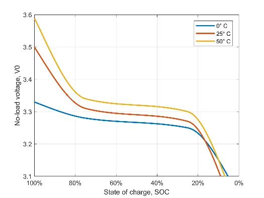
The Battery (Table-Based) block represents a high-fidelity battery model. The block calculates no-load voltage as a function of charge level and optional temperature using lookup tables and includes several modeling options:
-
Self-discharge
-
Battery fade
-
Charge dynamics
-
Calendar aging
Note
The block can use linear or nearest interpolation and extrapolation for all the table based parameters. For rows and columns, it follows the row-column convention, whereas rows are indexed first and, subsequently, columns.
The plot shows a battery whose performance varies with temperature and state of charge changes, as typically found on a datasheet.
Use this block to parameterize batteries with complex no-load voltage behavior from datasheets or experimental results. For a simpler representation of a battery, see the Battery block.
The Battery (Table-Based) block has four modeling variants, accessible by right-clicking the block in your block diagram and then selecting the appropriate option from the context menu, under Simscape > Block choices:
-
Uninstrumented | No thermal port — Basic model that does not output battery charge level and simulates at a fixed temperature. This modeling variant is the default.
-
Uninstrumented | Show thermal port — Model with exposed thermal port. This model does not output internal charge level of the battery.
-
Instrumented | No thermal port — Model with exposed charge output port. This model uses a fixed temperature throughout the simulation.
-
Instrumented | Show thermal port — Model that lets you output internal charge level of the battery. Both the thermal port and the charge output port are exposed.
The instrumented variants have an extra physical signal port that outputs the internal state of charge. Use this functionality to change load behavior as a function of state of charge, without the complexity of building a charge state estimator.
The thermal port variants expose a thermal port, which represents the battery thermal mass.
You can also choose different built-in parameterizations for this block. For more information, see the Predefined Parameterization section.
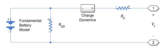
The battery equivalent circuit is made up of the fundamental battery model, the self-discharge resistance RSD, the charge dynamics model, and the series resistance R0.
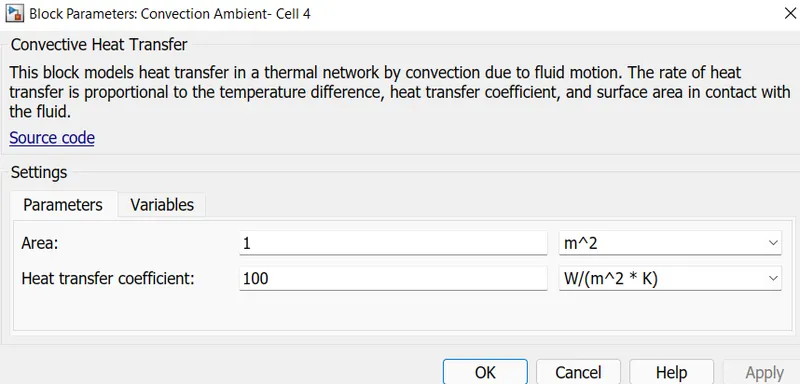
Convective Heat Transfer

The Convective Heat Transfer block represents a heat transfer by convection between two bodies by means of fluid motion. The transfer is governed by the Newton law of cooling and is described with the following equation:
Q=k·A·(TA−TB)
where
| Q | Heat flow |
| k | Convection heat transfer coefficient |
| A | Surface area |
| TA,TB | Temperatures of the bodies |
Connections A and B are thermal conserving ports associated with the points between which the heat transfer by convection takes place. The block positive direction is from port A to port B. This means that the heat flow is positive if it flows from A to B.
Variables
To set the priority and initial target values for the block variables prior to simulation, use the Variables tab in the block dialog box (or the Variables section in the block Property Inspector). For more information, see Set Priority and Initial Target for Block Variables.
Parameters
- Area
-
Surface area of heat transfer. The default value is
1m^2. - Heat transfer coefficient
-
Convection heat transfer coefficient. The default value is
100W/m^2/K.
Ports
The block has the following ports:
AThermal conserving port associated with body A.BThermal conserving port associated with body B.
Conductive Heat Transfer
Heat transfer by conduction
Library
Thermal Elements.

Description
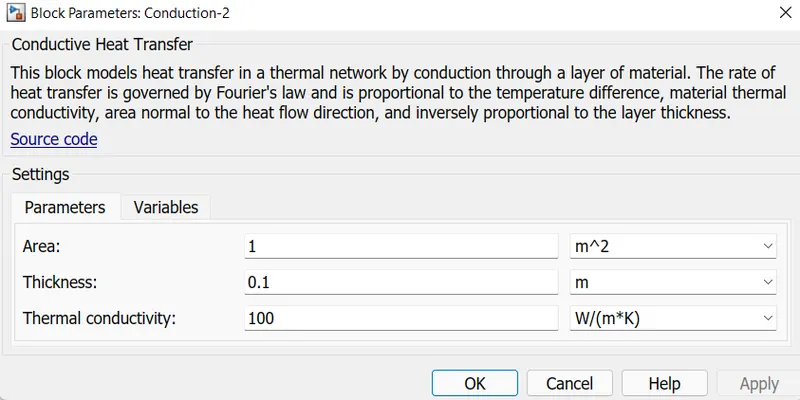
The Conductive Heat Transfer block represents a heat transfer by conduction between two layers of the same material. The transfer is governed by the Fourier law and is described with the following equation:
Q=k·AD(TA−TB)
where
| Q | Heat flow |
| k | Material thermal conductivity |
| A | Area normal to the heat flow direction |
| D | Distance between layers (thickness of material) |
| TA,TB | Temperatures of the layers |
Connections A and B are thermal conserving ports associated with material layers. The block positive direction is from port A to port B. This means that the heat flow is positive if it flows from A to B.
Variables
To set the priority and initial target values for the block variables prior to simulation, use the Variables tab in the block dialog box (or the Variables section in the block Property Inspector). For more information, see Set Priority and Initial Target for Block Variables.
Parameters
- Area
-
Area of heat transfer, normal to the heat flow direction. The default value is
1m^2. - Thickness
-
Thickness of material, that is, distance between layers. The default value is
0.1m. - Thermal conductivity
-
Thermal conductivity of the material. The default value is 100 W/m/K.
Ports
The block has the following ports:
AThermal conserving port associated with layer A.BThermal conserving port associated with layer B.
Temperature Source

Description
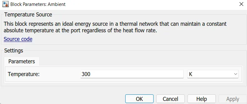
The Temperature Source block represents an ideal source of thermal energy that is powerful enough to maintain specified temperature at its outlet regardless of the heat flow consumed by the system.
The source generates constant absolute temperature, defined by the Temperature parameter value.
Ports
A — Source outlet thermal
AC Current Source
Ideal sinusoidal current source
Library
Electrical Sources

Description
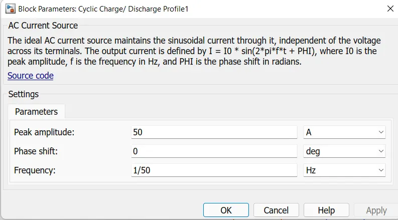
The AC Current Source block represents an ideal current source that maintains sinusoidal current through it, independent of the voltage across its terminals.
The output current is defined by the following equation:
I=I0⋅sin(2π⋅f⋅t+φ)
where
| I | Current |
| I0 | Peak amplitude |
| f | Frequency |
| φ | Phase shift |
| t | Time |
The positive direction of the current flow is indicated by the arrow.
Parameters
- Peak amplitude
-
Peak current amplitude. The value is 50A.
- Phase shift
-
Phase shift in angular units. The value is
0. - Frequency
-
Current frequency, specified in Hz or units directly convertible to Hz (where Hz is defined as
1/s). For example,kHzandMHzare valid units, butrad/sis not. The default value is50Hz.
Ports
The block has two electrical conserving ports associated with its terminals.
Temperature Sensor
Ideal temperature sensor
Library
Thermal Sensors

Description
The Temperature Sensor block represents an ideal temperature sensor, that is, a device that determines the temperature differential measured between two points without drawing any heat.
Connections A and B are thermal conserving ports that connect to the two points where temperature is being monitored. Port T is a physical signal port that outputs the temperature differential value.
The block positive direction is from port A to port B. The measured temperature is determined as T = TA – TB.
Ports
The block has the following ports:
AThermal conserving port associated with the sensor positive probe.BThermal conserving port associated with the sensor negative probe.TPhysical signal output port for temperature.
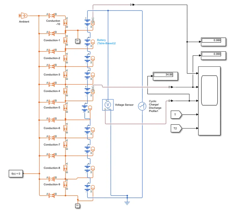
1. How the connection is made -10 lithium-ion battery cells are connected in with the combination.
2. the heat transfer is observed between the packs by conduction and convection block which are modes of heat transfer.
3. T subsystem is attached ini between every pack to plot the temperature groph of the cell of that particular battery pack
4. also external ambient temperature source is attached and also thermal sensor is attoched to the same to indicate the value in the display
5. this battery pack is connected to AC current source to observe the cyclic charge and discharge rate graph.
6. the cell temperoture and soc graphs are ploted in scope which indicating the temperature of cell no 1, cell no 5,
| SLNO | CASE | 1 TO 4 CELLES | 5 & 6CELLES | 7 TO 10 CELLES |
| 1 | CASE-1 | 298.15K | 298.15K | 298.15K |
| 2 | CASE-2 | 298.15K | 350K | 400K |
| 3 | CASE-3 | 298.15K | 400K | 450K |
CASE-1
| 1 | CASE-1 | 298.15K | 298.15K | 298.15K |
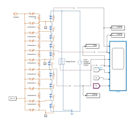
The above fig shows the For a 10 cell series lithium ion battery model, simulate the thermal effects and compare life cycle performance at various temperatures, charge & discharge rates using MATLAB.
the all battery are same temperature coefficient that is shown in above table.
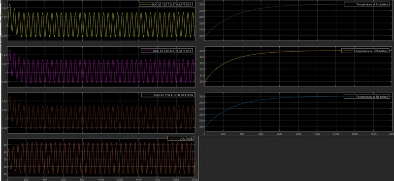
where For first 300 Secs our SOc reaches to 1.04 during charging then 300 secs for discharging with the same value, in one hour it has corpleted the 6 complete cycles with charging and discharging.
CASE-2
| 2 | CASE-2 | 298.15K | 350K | 400K |
and kept Ambient temperture is constant at 350k
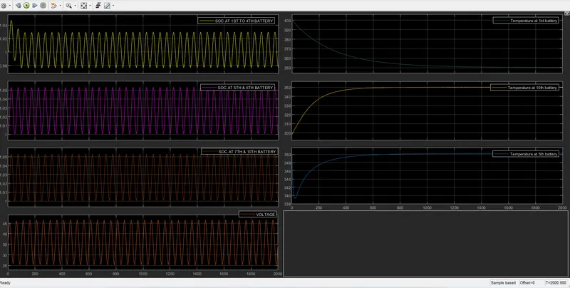
the above wave from show the output of the case -2 mension above table values are given to the battery temperature and remaining values are constant and also Ambient also constant 350k the wave from show the if battery temperature was increses also after some time battery tempereture reach Ambient temperature.
CASE-2
| 2 | CASE-3 | 298.15K | 400K | 450K |
and kept Ambient temperture is constant at 350k
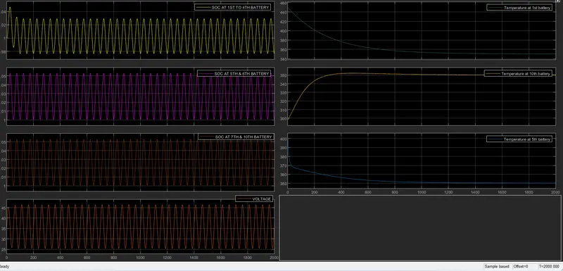
the above wave from show the output of the case -3 mension above table values are given to the battery temperature and remaining values are constant and also Ambient also constant 350k the wave from show the if battery temperature was increses also after some time battery tempereture reach Ambient temperature.