Challenge

Project 2 - Rankine cycle Simulator

GGuberan V26 May 2023

Aim

To create Rankine cycle simulator in matlab

Before we creating the program for rankine simulation first understand the concept of rankine cycle and its principle

Basic Cycle

The Rankine cycle is the fundamental operating cycle of all power plants where an operating fluid is continuously evaporated and condensed. The selection of operating fluid depends mainly on the available temperature range the idealized Rankine cycle it has four stages which

1-2-3 Isobaric Heat Transfer

3-4 Isentropic Expansion

4-5 Isobaric Heat Rejection

5-1 Isentropic Compression

these four stages are basic concept of the rankine cycle and have changed the input four method for the programing of rankine cycle simulation

1-2-3 Isobaric heat transfer

High pressure liquid enters the boiler from the feed pump (1) and is heated to the saturation temperature (2). Further addition of energy causes evaporation of the liquid until it is fully converted to saturated steam

3-4 isentropic expanssion

The vapor is expanded in the turbine, thus producing work which may be converted to electricity. In practice, the expansion is limited by the temperature of the cooling medium and by the erosion of the turbine blades by liquid entrainment in the vapor stream as the process moves further into the two-phase region. Exit vapor qualities should be greater than 90%

4-5 Isobaric heat rejection

The vapor-liquid mixture leaving the turbine (4) is condensed at low pressure, usually in a surface condenser using cooling water. In well designed and maintained condensers, the pressure of the vapor is well below atmospheric pressure, approaching the saturation pressure of the operating fluid at the cooling water temperature.

5-1 isentropic compression

The pressure of the condensate is raised in the feed pump. Because of the low specific volume of liquids, the pump work is relatively small and often neglected in thermodynamic calculations.

The thermal efficiency of power cycles is defined as

and the given formulas are used to find the respective functions in the model to identify its outputs

Turbine

t = h1-h2

for boiler

q1 = h1-h4

for condesor

q2 = h2-h3

and in pump

p = h4-h3

Inefficiencies of Real Rankine Cycles

The efficiency of the ideal Rankine cycle as described in the previous section is close to the Carnot efficiency In real plants, each stage of the Rankine cycle is associated with irreversible processes, reducing the overall efficiency. Turbine and pump irreversibilities can be included in the calculation of the overall cycle efficiency by defining a turbine efficiency

Program file

clear all

close all

clc

% Considering the inputs of the

% 1 = Turbine inlet, 3 = Condenser inlet,

% 2 = Pump inlet, 4 = Boiler inlet

% p1 = Turbine inlet pressure (bar),

% T1 = Temperature at turbine inlet(deg C),

% p2 = Turbine outlet pressure (bar),

% four process inside of ,

fprintf('Process (1-2) - Isentropic Expansion in the Turbine\n')

fprintf('Process (2-3) - Isobaric Heat Rejection by the Condenser\n')

fprintf('Process (3-4) - Isentropic Compression in the Pump\n')

fprintf('Process (4-1) - Isobaric Heat Addition by the Boiler\n')

% inputs variables for state point 1,

p_in = input('Enter the Pressure at the Turbine Inlet (in bar): ');

t1 = input('Enter the Temperature at the Turbine inlet (in Degree celsius): ');

p_out = input('Enter the Pressure at the Turbine Outlet (in bar): ');

% variables for State point 1

% Enthalpy in [kJ/kg]

h1 = XSteam('h_pT',p_in,t1);

% Specific entropy in [kJ/kg K]

s1 = XSteam('s_pT',p_in,t1);

% Specific volume in [m3/kg]

v1 = XSteam('v_pT',p_in,t1);

% variavle for State point 2

% Specific entropy in [kJ/kg K]

s2 = s1;

% Enthalpy in [kJ/kg]

h2 = XSteam('h_px',p_out,XSteam('x_ps',p_out,s2));

% Temperature in [degree C]

t2 = XSteam('T_ps',p_out,s2);

% Specific volume in [m3/kg]

v2 = XSteam('v_ps',p_out,s2);

% variable for State point 3

% Pressure in [bar]

p3 = p_out;

% Temperature in [degree C]

t3 = XSteam('Tsat_p',p3);

% Enthalpy in [kJ/kg]

h3 = XSteam('hL_p',p3);

% Specific entropy in [kJ/kg K]

s3 = XSteam('sL_p',p3);

% Inlet Specific volume in [m3/kg]

v3 = XSteam('vL_p',p3);

%variable for State point 4

% Specific entropy in [kJ/kg K]

s4 = s3;

% Pressure in [bar]

p4 = p_in;

% Enthalpy in [kJ/kg]

h4 = XSteam('h_ps',p4,s4);

% Temperature in [degree C]

t4 = XSteam('T_ps',p4,s4);

% Specific volume in [m3/kg]

v4 = XSteam('v_ps',p4,s4);

% Ploting

figure(1)

hold on

plot([s1 s2],[t1 t2],'color','r');

plot([s2 s3],[t2 t3],'color','k');

plot([s3 s4],[t3 t4],'color','c');

Trange = linspace(t4,t1,500);

for i = 1:length(Trange)

s_range(i) = XSteam('s_pT',p_in,Trange(i));

h_range23(i) = XSteam('h_ps',p_in,s_range(i));

h_range41(i) = XSteam('h_ps',p_out,s_range(i));

end

plot(s_range,Trange,'color','c');

figure(2)

hold on

plot([s1 s2],[h1 h2],'color','b');

plot(s_range,h_range23,'color','k');

plot([s3 s4],[h3 h4],'color','c');

plot(s_range,h_range41,'color','g');

t_range = linspace(0,374.15,100);

figure(1)

hold on

for i = 1:length(t_range)

plot(XSteam('sV_t',t_range(i)))

end

figure(2)

hold on

for i = 1:length(t_range)

plot(XSteam('sL_t',t_range(i)),XSteam('hL_t',t_range(i)),'color','k')

plot(XSteam('sV_t',t_range(i)),XSteam('hV_t',t_range(i)),'color','r')

end

%Ideal Rankine cycle in 'T' vs 's'

figure(1)

hold on

plot(s1,t1)

plot(s2,t2)

plot(s3,t3)

plot(s4,t4)

grid on

title('t-s Diagram of RANKINE CYCLE')

xlabel('Temperature in [degree C]')

ylabel('Specific entropy in [kJ/kg K]')

figure(2)

hold on

plot(s1,h1)

plot(s2,h2)

plot(s3,h3)

plot(s4,h4)

grid on

title('h-s Diagram of RANKINE CYCLE')

xlabel('Enthalpy in [kJ/kg]')

ylabel('Specific entropy in [kJ/kg K]')

% to calculate Work and Efficiency

Work_turbine = h1 - h2;

Q_taken_out_condenser = h2 - h3;

Work_pump = h4 - h3;

Q_given_boiler = h1 - h4;

Back_Work_Ratio = Work_turbine / Work_pump;

SSE = 3600/(Work_turbine - Work_pump);

Work_net = Work_turbine - Work_pump;

Effi_rankine = Work_net/Q_given_boiler;

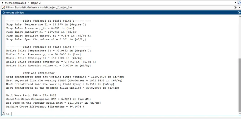
clc

% results for the inputs given

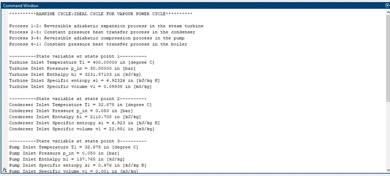
fprintf('**********RANKINE CYCLE:IDEAL CYCLE FOR VAPOUR POWER CYCLE**********\n\n');

fprintf('Process 1-2: Reversible adiabatic expansion process in the steam turbine\n');

fprintf('Process 2-3: Constant pressure heat transfer process in the condenser\n');

fprintf('Process 3-4: Reversible adiabatic compression process in the pump\n');

fprintf('Process 4-1: Constant pressure heat transfer process in the boiler\n\n');

fprintf('----------State variable at state point 1----------\n');

fprintf('Turbine Inlet Temperature T1 = %.5f in [degree C]\n',t1);

fprintf('Turbine Inlet Pressure p_in = %.5f in [bar]\n',p_in);

fprintf('Turbine Inlet Enthalpy h1 = %.5f in [kJ/kg]\n',h1);

fprintf('Turbine Inlet Specific entropy s1 = %.5f in [kJ/kg K]\n',s1);

fprintf('Turbine Inlet Specific volume v1 = %.5f in [m3/kg]\n\n',v1);

fprintf('----------State variable at state point 2----------\n');

fprintf('Conderser Inlet Temperature T1 = %.3f in [degree C]\n',t2);

fprintf('Conderser Inlet Pressure p_in = %.3f in [bar]\n',p_out);

fprintf('Conderser Inlet Enthalpy h1 = %.3f in [kJ/kg]\n',h2);

fprintf('Conderser Inlet Specific entropy s1 = %.3f in [kJ/kg K]\n',s2);

fprintf('Conderser Inlet Specific volume v1 = %.3f in [m3/kg]\n \n',v2);

fprintf('----------State variable at state point 3----------\n');

fprintf('Pump Inlet Temperature T1 = %.3f in [degree C]\n',t3);

fprintf('Pump Inlet Pressure p_in = %.3f in [bar]\n',p3);

fprintf('Pump Inlet Enthalpy h1 = %.3f in [kJ/kg]\n',h3);

fprintf('Pump Inlet Specific entropy s1 = %.3f in [kJ/kg K]\n',s3);

fprintf('Pump Inlet Specific volume v1 = %.3f in [m3/kg]\n\n',v3);

fprintf('----------State variable at state point 4----------\n');

fprintf('Boiler Inlet Temperature T1 = %.4f in [degree C]\n',t4);

fprintf('Boiler Inlet Pressure p_in = %.4f in [bar]\n',p4);

fprintf('Boiler Inlet Enthalpy h1 = %.4f in [kJ/kg]\n',h4);

fprintf('Boiler Inlet Specific entropy s1 = %.4f in [kJ/kg K]\n',s4);

fprintf('Boiler Inlet Specific volume v1 = %.4f in [m3/kg]\n \n',v4);

fprintf('----------Work and Efficiency----------\n');

fprintf('Work transferred from the working fluid Wturbine = %.4f in [kJ/kg]\n',Work_turbine);

fprintf('Heat rejected from the working fluid Qcondenser = %.4f in [kJ/kg]\n',Q_taken_out_condenser);

fprintf('Work transferred into the working fluid Wpump = %.4f in [kJ/kg]\n',Work_pump);

fprintf('Heat transferred to the working fluid Qboiler = %.4f in [kJ/kg]\n \n',Q_given_boiler);

fprintf('Back Work Ratio BWR = %.4f \n',Back_Work_Ratio);

fprintf('Specific Steam Consumption SSE = %.4f in [kg/kWh] \n',SSE);

fprintf('Net work on the working fluid Wnet = %.4f in [kJ/kg] \n',Work_net);

fprintf('Rankine Cycle Efficiency ETArankine = %.4f %% \n\n',Effi_rankine*100);

Explanation

In this program the inputs are taken as given in the challenge as

Turbine Inlet temperature = 400° C

Turbine Inlet Pressure = 30 bars

Turbine Outlet Pressure = 0.05 bars = Condenser Inlet Pressure with this inputs we can create a program for the 4 function which taken randomly as

(1-2) - Isentropic Expansion in the Turbine\n')

(2-3) - Isobaric Heat Rejection by the Condenser\n')

(3-4) - Isentropic Compression in the Pump\n')

(4-1) - Isobaric Heat Addition by the Boiler\n')

after given the four functions we have to identify the enthalpy,entropy,specific volume and heat of the state points and work efficiency of the model and we can get the input variables from the xsteam library for the datas for water

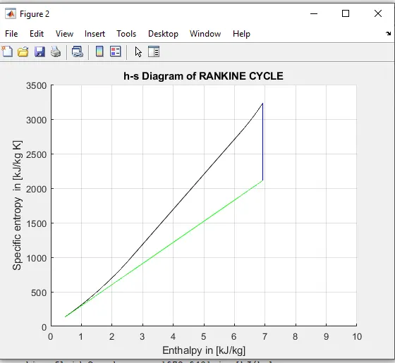
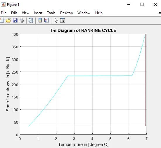
after that we can plot the figure for t-s,h-s and the work and efficiency are calculated using the inputs given and the results can be printed in command windoe using Prinf command for the 4 state points

Outputs

Ploted figures for the H-S

Ploted figure for T-S

Project 2 - Rankine cycle Simulator

Basic Cycle

Ship work like this
in your own course.

Talk to a career counsellor

Basic Cycle

Ship work like thisin your own course.

Talk to a career counsellor

Ship work like this
in your own course.