%% Skill-Lync -> Hybrid Drives Development
% Project 1 - Conventional Vehicle Model
% By - Guberan
% Description:
% The following file is to used with the Initialization file and Simulink
% results for post-processing of the data.
% The file is incomplete, has some examples of how the data is imported
% into a readable format, data analysis and plotting examples.
% Based on the project task, use commands in a similar format as given
% below, to analyse the data and generate required plots.
% You can change variable names if desired
%% Post-Processing File
% File for post-processing the Conventional vehicle simulation model data
%% Renaming variables
Time = out.tout;
Acc_Pdl = out.Acc_Pdl; % Accelerator pedal [%]
Brake_Pdl = out.Brk_Pdl; % Brake pedal [%]
Gear_Cmd = out.Gear_Cmd; % Transmission gear
Trans_In_Spd = out.Trans_In_Spd*30/pi; % Transmission input speed [rpm]
Trans_Out_Spd = out.Trans_Out_Spd*30/pi;% Transmission output speed [rpm]
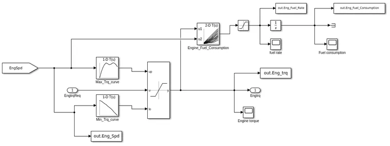
Eng_Trq = out.Eng_trq; % Engine brake torque [Nm]
Eng_Spd = out.Eng_Spd*30/pi; % Engine speed [rpm]
Eng_Fuel_Consump = out.Eng_Fuel_Consumption; % Engine fuel consumption [g]
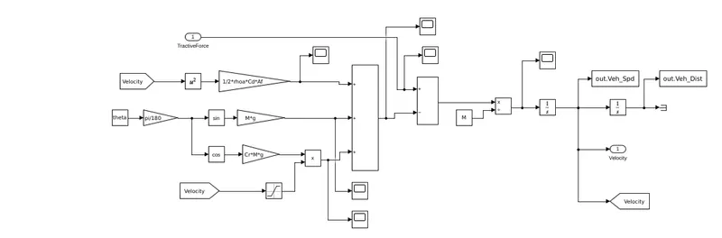
Veh_Dist = out.Veh_Dist/1000; % Distance traveled by vehicle [km]
Veh_Spd = out.Veh_Spd*18/5; % Vehicle speed [kmph]
Eng_Fuel_Rate = out.Eng_Fuel_Rate; % Engine fuel rate
%% Data Analysis
Eng_Pwr = Eng_Spd*pi/30*Eng_Trq/1000; % Engine brake power [kW]
rho_petrol = 0.7197; % Density of petrol [kg/L]
kmpl = Veh_Dist(end)/(Eng_Fuel_Consump(end)/1000/rho_petrol); % Fuel economy [kmpl]
%% Plotting vehicle characteristics time trace
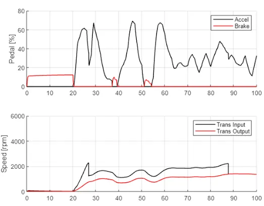
figure(1)
subplot(2,1,1)
hold on
grid on
plot (Time, Acc_Pdl, 'linewidth', 1, 'Color', 'black');
plot(Time, Brake_Pdl, 'linewidth', 1, 'Color', 'red');
ylabel('Pedal [%]')
xlim([0, Time(end)]);
legend('Accel','Brake');
subplot(2,1,2)
hold on
grid on
plot(Time, Trans_In_Spd, 'linewidth', 1, 'Color', 'black');
plot(Time, Trans_Out_Spd, 'linewidth', 1, 'Color', 'red');
ylabel('Speed [rpm]')
xlim([0, Time(end)]);
ylim([0, 6000]);
legend('Trans Input','Trans Output','wheel speed');
%plotting vehicle charecterstics timetrace to engine torque,fuel consumption,fuel rate and engine
%speed
%data converstion from doubletimeseries
Eng_spd = Eng_Spd.Data(:,1); % engine speed
Eng_Trq = Eng_Trq.Data(:,1); %engine torque
Eng_Pwr = Eng_Pwr.Data(:,1); %engine power
Eng_Fuel_Consumption = Eng_Fuel_Consump.Data(:,1); % fuel_consumption
Eng_Fuel_Rate = Eng_Fuel_Rate.Data(:,1); % engine Fuel_rate
Veh_Spd = Veh_Spd.Data(:,1); %Veh_spd
Veh_Dist = Veh_Dist.Data(:,1); %Vehicle distance
%plotting Engine Torque,Fuel consumption,Power,fuel rate
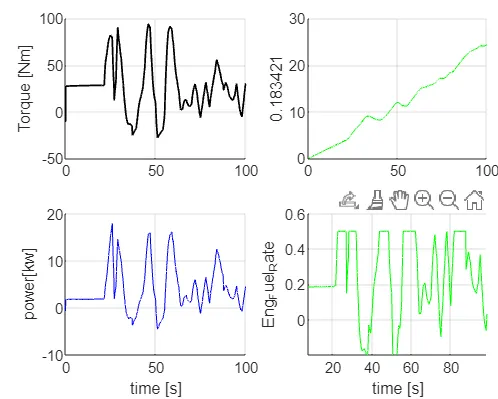
figure (2)
subplot(2,2,1)
hold on
grid on
plot(Time,Eng_Trq, 'linewidth', 1, 'Color', 'black');
ylabel('Torque [Nm]')
xlim([0, Time(end)]);
subplot(2,2,2)
hold on
grid on
plot(Time,Eng_Fuel_Consumption,'g');
xlim([0, Time(end)]);
ylabel(Eng_Fuel_Consumption('g'));
subplot (2,2,3)
hold on
grid on
plot(Time,Eng_Pwr,'b');
xlim([0,Time(end)]);
xlabel('time [s]');
ylabel('power[kw]');
subplot (2,2,4)
hold on
grid on
plot (Time,Eng_Fuel_Rate,'g');
xlim([0,Time(end)]);
xlabel('time [s]');
ylabel('Eng_Fuel_Rate');
%ploting accelerator and brake pedal, gear command, vehicle desired and actual speed, vehicle distance
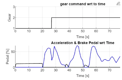
figure(3)
subplot(3,1,1)
hold on
grid on
plot(Time, Gear_Cmd, 'linewidth', 1, 'Color', 'black');
xlim([0, Time(end)]);
xlabel('Time [s]');
ylabel('Gear');
grid on
title('gear command wrt to time')
subplot(3,1,2)
hold on
plot(Time, Acc_Pdl, 'linewidth', 1, 'color','b');
xlabel('Time [s]');
xlim([0, Time(end)]);
plot(Time, Brake_Pdl, 'linewidth', 1, 'Color', 'k');
ylabel('Pedal [%]');
title('aaceleration wrt to time');
grid on
legend('Accel','Brake');
title('Acceleration & Brake Pedal wrt Time')
%ploting vehice speed and actual speed
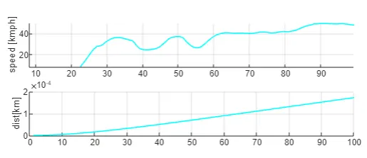
figure(4)
subplot(4,1,1)
hold on
grid on
plot(Time,Veh_Spd, 'linewidth', 1, 'Color','c');
xlim([0, Time(end)]);
xlim([0, Time(end)]);
ylabel('speed [kmph]');
subplot(4,1,2)
hold on
grid on
plot(Veh_Dist, 'linewidth', 1, 'Color','c');
xlim([0, Time(end)]);
ylabel('dist[km]');
%ploting for drive cycles
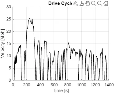
figure(5)
hold on
grid on
plot(cyc_time, cyc_vel, 'linewidth', 1, 'Color', 'black');
xlabel('Time [s]')
ylabel('Velocity [Mph]')
title('Drive Cycle')
% Test Results
Avg_speed = sum(Veh_Spd)/length(Veh_Spd);
Max_Speed = maxk(Veh_Spd,1);
table(Avg_speed,Max_Speed,kmpl,'VariableNames',{'Average Speed [kmph]','Maximum Speed [kmph]','Fuel Economy [kmpl]'})
%% Plotting engine operating points on engine fuel map
figure('Name','Engine Operating Points');
hold on
grid on
title('Engine Operating Points','fontsize',12);
p1=plot(Eng_map_spd*30/pi,Eng_max_trq,'linewidth',2,'color','r');
p2=line([Eng_map_spd(end)*30/pi Eng_map_spd(end)*30/pi],[0 Eng_max_trq(end)]);
set(p2,'linewidth',1,'linestyle','--','color','k');
p3=line([Eng_map_spd(1)*30/pi Eng_map_spd(1)*30/pi],[0 Eng_max_trq(1)]);
set(p3,'linewidth',1,'linestyle','--','color','k');
[c,h] = contour(Eng_map_spd'*30/pi,Eng_map_trq,Eng_fuel_map');
clabel(c,h);
xlabel('Engine Speed [rpm]');
ylabel('Engine Torque [Nm]');
title('Engine Fuel Consumption Map [g/s]');
legend([p1 p3],{'Max Curve','Operating Points'});
axis([Eng_map_spd(1)*30/pi Eng_map_spd(end)*30/pi 0 Eng_map_trq(end)]);