Project 2 - Rankine cycle Simulator

• The program first depicts the processes involved in the rankine cycle.
• State 1 and 2 pressures, as well as state 1 temperature, are read from the user.
• The Xsteam library values are extracted, and state values such as pressure, temperature, enthalphy, and entropy are determined.
• Turbine work, pump work, net work, thermal efficiency, back work ratio, and specific steam conductivity are also computed.
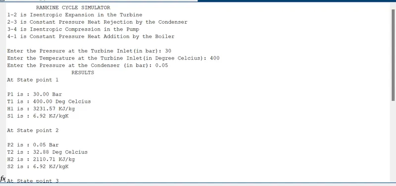
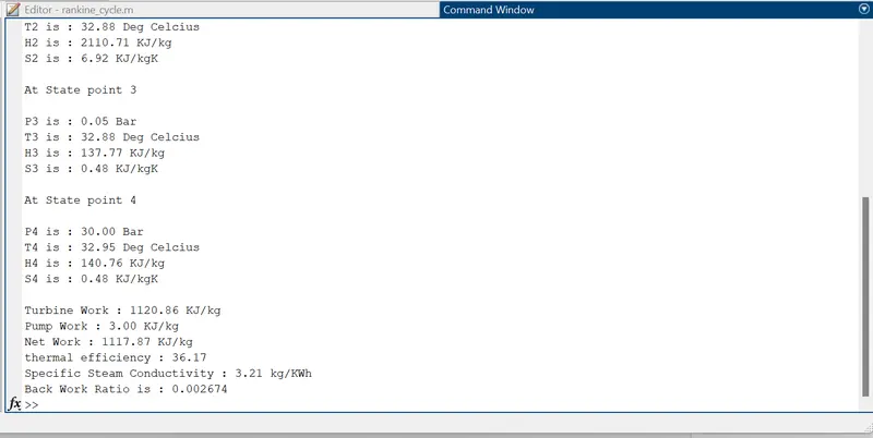
• The command window displays all of the computed values using the following formulas,
• Turbine Work (W_T) = H1 - H2

  Pump Work (W_P) = H4 - H3

  Net Work (W_NET) = W_T - W_P

  Thermal Efficiency of the Rankine Cycle (EFF) = (W_NET/(H1 - H4))*100

  Back Work Ratio (BWR)= W_P/W_T
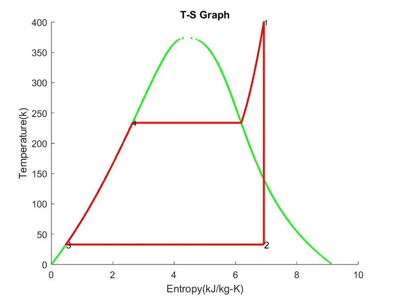
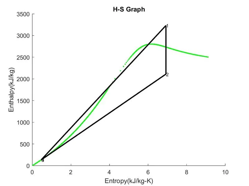
• Finally, the Rankine Cycle's T-S and H-S graphs are presented.

clear
close all
clc
disp('         RANKINE CYCLE SIMULATOR          ');
disp('1-2 is Isentropic Expansion in the Turbine');
disp('2-3 is Constant Pressure Heat Rejection by the Condenser');
disp('3-4 is Isentropic Compression in the Pump');
disp('4-1 is Constant Pressure Heat Addition by the Boiler');
fprintf('\n');

%Taking inputs from user
P1 = input('Enter the Pressure at the Turbine Inlet(in bar): ');
T1 = input('Enter the Temperature at the Turbine Inlet(in Degree Celcius): ');
P2 = input('Enter the Pressure at the Condenser (in bar): ');
%calculating state values 

%At state point 1
H1 = XSteam('h_pT',P1,T1);
S1 = XSteam('s_pT',P1,T1);
H_L1 = XSteam('hL_p',P1);
H_G1 = XSteam('hV_p',P1);
S_L1 = XSteam('sL_p',P1);
S_G1 = XSteam('sV_p',P1);
T_sat1 = XSteam('Tsat_p',P1);

%At state point 2
S2 = S1;
S_L2 = XSteam('sL_p',P2);
S_G2 = XSteam('sV_p',P2);
X = (S2-S_L2)/(S_G2-S_L2); %Calculating the dryness fraction
H_L2 = XSteam('hL_p',P2);
H_G2 = XSteam('hV_p',P2);
H2 = H_L2 + X*(H_G2 - H_L2);  %Calculating the enthalpy at point 2
T2 = XSteam('T_ph',P2,H2);
T_sat2 = XSteam('Tsat_p',P2);

%At state point 3
P3 = P2;
T3 = T2;
H3 = H_L2;
S3 = S_L2;

%At state point 4
P4 = P1;
S4 = S3;
T4 = XSteam('T_ps',P4,S4);
H4 = XSteam('H_ps',P4,S4);
%Turbine Work
W_T = H1 - H2;

%Pump Work
W_P = H4 - H3;

%Net Work
W_NET = W_T - W_P;

%Thermal Efficiency of the Rankine Cycle
EFF = (W_NET/(H1 - H4))*100 ;

%Back Work Ratio
BWR = W_P/W_T;

%Specific Steam Conductivity
SSC = 3600/W_T;
%Displaying results
%state point 1
disp('                    RESULTS                ');
disp('At State point 1');
fprintf('\nP1 is : %.2f Bar \n',P1);
fprintf('T1 is : %.2f Deg Celcius \n',T1);
fprintf('H1 is : %.2f KJ/kg \n',H1);
fprintf('S1 is : %.2f KJ/kgK \n\n',S1);
%Values of state point 2
disp('At State point 2');
fprintf('\nP2 is : %.2f Bar \n',P2);
fprintf('T2 is : %.2f Deg Celcius \n',T2);
fprintf('H2 is : %.2f KJ/kg \n',H2);
fprintf('S2 is : %.2f KJ/kgK \n\n',S2);

%Values of state point 3
disp('At State point 3');
fprintf('\nP3 is : %.2f Bar \n',P3);
fprintf('T3 is : %.2f Deg Celcius \n',T3);
fprintf('H3 is : %.2f KJ/kg \n',H3);
fprintf('S3 is : %.2f KJ/kgK \n\n',S3);

%Values of state point 4
disp('At State point 4');
fprintf('\nP4 is : %.2f Bar \n',P4);
fprintf('T4 is : %.2f Deg Celcius \n',T4);
fprintf('H4 is : %.2f KJ/kg \n',H4);
fprintf('S4 is : %.2f KJ/kgK \n',S4);

%Turbine Work
fprintf('\nTurbine Work : %.2f KJ/kg \n',W_T);

%Pump Work
fprintf('Pump Work : %.2f KJ/kg \n',W_P);

%Net Work
fprintf('Net Work : %.2f KJ/kg \n',W_NET);

%Thermal Efficiency
fprintf('thermal efficiency : %.2f %',EFF);

%Specific Steam Conductivity
fprintf('\nSpecific Steam Conductivity : %.2f kg/KWh \n',SSC);

%Back Work ratio
fprintf('Back Work Ratio is : %f \n',BWR);
%plotting of T-S curve
t = linspace(0,373.5,200);
figure(1)
hold on

for i = 1:length(t)
plot(XSteam('sL_T',t(i)),t(i),'g.')
plot(XSteam('sV_T',t(i)),t(i),'g.')
end

plot([S1 S2],[T1 T2],'linewidth',2,'color','r')
text(S1,T1,'1','FontSize',5)
if X>1
T3 = T_sat2;
plot([S2 S_G2 S3 S4],[T2 T_sat2 T3 T4],'linewidth',2,'color','r')
T2 = T_sat2;
text(S2,T2,'2','FontSize',5)
text(S3,T3,'3','FontSize',5)
else
plot([S2 S3 S4],[T2 T3 T4],'linewidth',2,'color','r')
text(S2,T2,'2','FontSize',10)
text(S3,T3,'3','FontSize',10)
end

n = linspace(T1,T2,500);
for i = 1:length(n)
plot(XSteam('s_pT',P1,n(i)),n(i),'.','linewidth',2,'color','r')
end

plot([S_L1 S_G1],[T_sat1 T_sat1],'linewidth',2,'color','r')
text(S_L1,T_sat1,'4','FontSize',5)
xlabel('Entropy(kJ/kg-K)')
ylabel('Temperature(k)')
title('T-S Graph')


%Plotting of H-S Curve
figure(2) 
hold on
for i = 1:length(t)
 plot(XSteam('sL_T',t(i)),XSteam('hL_T',t(i)),'g.')
 plot(XSteam('sV_T',t(i)),XSteam('hV_T',t(i)),'g.')
end
plot([S1 S2 S3 S4 S1],[H1 H2 H3 H4 H1],'linewidth',2,'color','k')
text(S1,H1,'1','FontSize',5)
text(S2,H2,'2','FontSize',5)
text(S3,H3,'3','FontSize',5)
text(S4,H4,'4','FontSize',5)
xlabel('Entropy(kJ/kg-K)')
ylabel('Enthalpy(kJ/kg)')
title('H-S Graph')

Note: No major error faced during programming