Project 2 - Rankine cycle Simulator

# Problem statement;

Understand the concept of Rankine cycle by referring to standard thermal engineering text book.

• Create a Rankine Cycle Simulator using OCTAVE/MATLAB.
• Your code should calculate the state points of the Rankine Cycle (any type of your choice) based on user inputs.
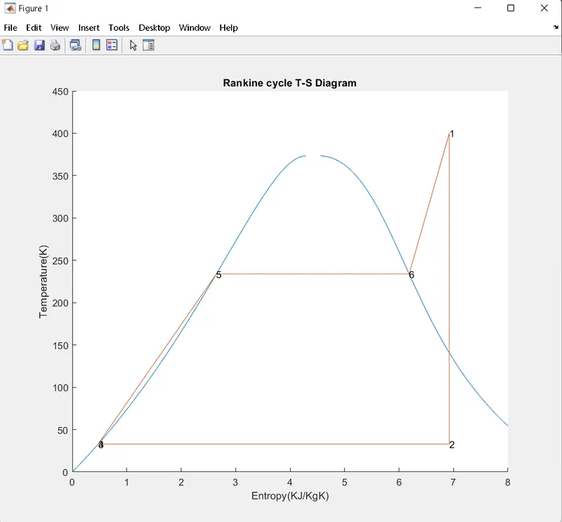
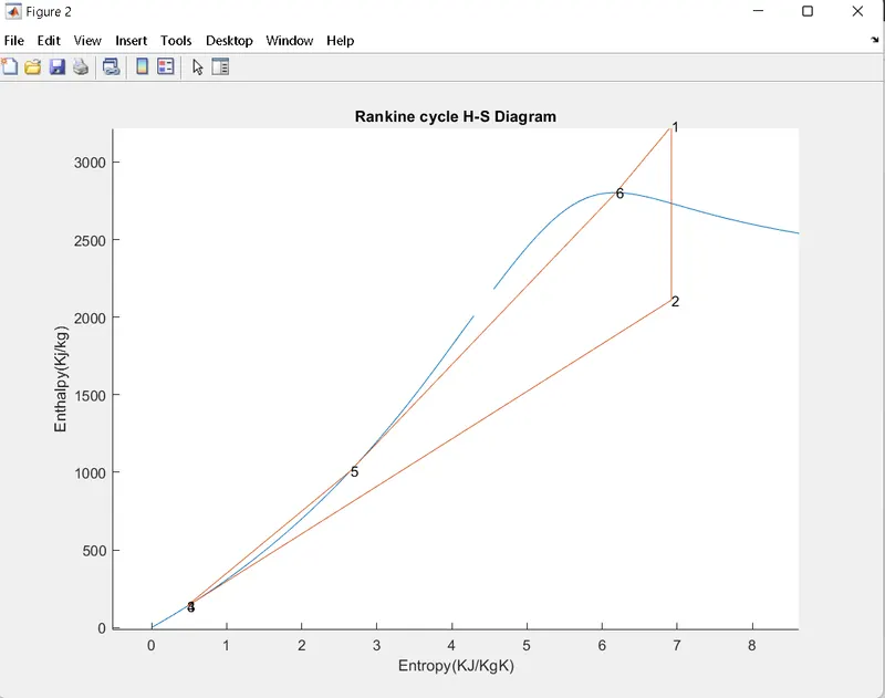
• Then, plot the corresponding T-s and h-s plots for the given set of inputs. Title and axes labels are a must, while legends could be used if necessary.
• The presentation of your code will be taken into consideration while grading. Labelling sections of your code using comments is appreciated.
• Attach a report explaining the working of a rankine cycle simulator and also the research done by you.

Contents expected in the report:

• Step-wise explanation of your code.
• Mention the errors faced while programming.
• Steps taken to overcome those errors.
• Screenshots showing errors thrown in command window.

# Rankine cycle;

The Rankine cycle is an idealized thermodynamic cycle describing the process by which certain heat engines, such as steam turbines or reciprocating steam engines, allow mechanical work to be extracted from a fluid as it moves between a heat source and heat sink. The Rankine cycle is named after William John Macquorn Rankine, a Scottish polymath professor at Glasgow University.

Heat energy is supplied to the system via a boiler where the working fluid (typically water) is converted to a high pressure gaseous state (steam) in order to turn a turbine. After passing over the turbine the fluid is allowed to condense back into a liquid state as waste heat energy is rejected before being returned to boiler, completing the cycle. Friction losses throughout the system are often neglected for the purpose of simplifying calculations as such losses are usually much less significant than thermodynamic losses, especially in larger systems.

The four processes in the Rankine cycle

There are four processes in the Rankine cycle. The states are identified by numbers (in brown) in the T–s diagram.

• Process 1–2: The working fluid is pumped from low to high pressure. As the fluid is a liquid at this stage, the pump requires little input energy. Process 1-2 is isentropic compression.
• Process 2–3: The high-pressure liquid enters a boiler, where it is heated at constant pressure by an external heat source to become a dry saturated vapour. The input energy required can be easily calculated graphically, using an enthalpy–entropy chart (h–s chart, or Mollier diagram), or numerically, using steam tables or software. Process 2-3 is constant pressure heat addition in boiler.
• Process 3–4: The dry saturated vapour expands through a turbine, generating power. This decreases the temperature and pressure of the vapour, and some condensation may occur. The output in this process can be easily calculated using the chart or tables noted above. Process 3-4 is isentropic expansion.
• Process 4–1: The wet vapour then enters a condenser, where it is condensed at a constant pressure to become a saturated liquid. Process 4-1 is constant pressure heat rejection in condenser.

In an ideal Rankine cycle the pump and turbine would be isentropic, i.e., the pump and turbine would generate no entropy and hence maximize the net work output. Processes 1–2 and 3–4 would be represented by vertical lines on the T–s diagram and more closely resemble that of the Carnot cycle. The Rankine cycle shown here prevents the state of the working fluid from ending up in the superheated vapor region after the expansion in the turbine, ^[1] which reduces the energy removed by the condensers.

The actual vapor power cycle differs from the ideal Rankine cycle because of irreversibilities in the inherent components caused by fluid friction and heat loss to the surroundings; fluid friction causes pressure drops in the boiler, the condenser, and the piping between the components, and as a result the steam leaves the boiler at a lower pressure; heat loss reduces the net work output, thus heat addition to the steam in the boiler is required to maintain the same level of net work output.

Variables

	Heat flow rate to or from the system (energy per unit time)
	Mass flow rate (mass per unit time)
	Mechanical power consumed by or provided to the system (energy per unit time)
	Thermodynamic efficiency of the process (net power output per heat input, dimensionless)
	Isentropic efficiency of the compression (feed pump) and expansion (turbine) processes, dimensionless
	The "specific enthalpies" at indicated points on the T–s diagram
	The final "specific enthalpy" of the fluid if the turbine were isentropic
	The pressures before and after the compression process

Equations

In general, the efficiency of a simple rankine cycle can be written as

Each of the next four equations^[1] is derived from the energy and mass balance for a control volume. �therm defines the thermodynamic efficiency of the cycle as the ratio of net power output to heat input. As the work required by the pump is often around 1% of the turbine work output, it can be simplified.

When dealing with the efficiencies of the turbines and pumps, an adjustment to the work terms must be made:

code for rankine cycle;

clear all
close all
clc

disp("         Rankine cycle simulator");
fprintf('\n 1-2  is the  isentropic expansion process');
fprintf('\n 2-3  is the constant pressure heat rejection process');
fprintf('\n 3-4  is the isentropic compression process');
fprintf('\n 4-1  is the constant pressure heat addition process');

% 
% T1 = 400;
% p1 = 30;
% p2 = 0.05;


% Required Inputs by user
p1 = input("Enter the Pressure at the Turbine inlet(in bar) = ");
T1 = input("Enter the Temperature at the Turbine inlet(in degree celcius) = ");
p2 = input("Enter the Pressure at the condenser(in bar) = ");
disp(' ')

 p4 = p1;
 p3 = p2;

S_liquid1 = XSteam('sL_p',p1);

S_gas1 = XSteam('sV_p',p1);
sf2 = XSteam('sL_p',p2);
sv2 = XSteam('sV_p',p2);
sf3 = XSteam('sL_p',p2);

T_saturation1 = XSteam('Tsat_p',p1);
T_saturation2 = XSteam('Tsat_p',p2);

h1 = XSteam('h_pt',p1,T1);

s1  = XSteam('s_pT',p1,T1);

s2 = s1;
% dryness fraction 

x2 = (s2-sf3)/(sv2-sf3);
hf2 = XSteam('hL_p',p2);
hg2 = XSteam('hV_p',p2);
h2 = hf2 + x2*(hg2-hf2);
% work obtained by the turbine

W_t = h1 - h2;
h3 = XSteam('hL_p',p2);
s3 = sf3;
s4 = s3;
h4 = XSteam('h_ps',p1,s4);

% work done on pump
 W_p = h4 -h3;

 % net work putput

 W_net = W_t - W_p;

 % back work ratio is given by the ratio of negative work that is pump work
 % to the positive work that is turbine

 back_work_ratio = W_p/W_t;

 % heat supplied to the boiler Q_s

 Q_s = h1 - h4;

 % heat rejected from the condensor

 Q_r = h2 - h3;

 % properties at point 1 are

 fprintf('properties at state point %d are',1);
 fprintf(' \n pressure (p1) at point 1 = %f in bar',p1);
 fprintf('\n temperature(T1) at point 1 = %f in Deg celcious',T1);
 fprintf('\n enthalpy(h1) at point 1 = %f in kj/kg',h1);
 fprintf('\n entropy(s1) at point 1 = %f in kj/kgk',s1);


 % properties at point 2 are

 T2 = XSteam('T_ps',p2,s2);

 fprintf('properties at state point %d are',2);
 fprintf(' \n pressure (p2) at point 2 = %f in bar',p2);
 fprintf('\n temperature(T2) at point 2 = %f in Deg celcious',T2);
 fprintf('\n enthalpy(h2) at point 2 = %f in kj/kg',h2);
 fprintf('\n entropy(s2) at point 2 = %f in kj/kgk',s2);


  % properties at point 3 are
  T3 = XSteam('T_ps',p3,s3);

 fprintf('properties at state point %d are',3);
 fprintf(' \n pressure (p3) at point 3 = %f in bar',p3);
 fprintf('\n temperature(T3) at point 3 = %f in Deg celcious',T3);
 fprintf('\n enthalpy(h3) at point 3 = %f in kj/kg',h3);
 fprintf('\n entropy(s3) at point 3 = %f in kj/kgk',s3);

  % properties at point 4 are

  T4 = XSteam('T_ps',p4,s4);
 fprintf('properties at state point %d are',4);
 fprintf(' \n pressure (p4) at point 4 = %f in bar',p4);
 fprintf('\n temperature(T4) at point 4 = %f in Deg celcious',T4);
 fprintf('\n enthalpy(h4) at point 4 = %f in kj/kg',h4);
 fprintf('\n entropy(s4) at point 4 = %f in kj/kgk',s4);

 % properties at point 6 are

 p6 = p1;
 T6 = XSteam('Tsat_p',p1);
 s6 = XSteam('sV_p',p1);
 h6 = XSteam('hV_p',p1);

 fprintf('properties at state point %d are',6);
 fprintf(' \n pressure (p6) at point 6 = %f in bar',p6);
 fprintf('\n temperature(T6) at point 6 = %f in Deg celcious',T6);
 fprintf('\n enthalpy(h6) at point 6 = %f in kj/kg',h6);
 fprintf('\n entropy(s6) at point 6 = %f in kj/kgk',s6);
 

% properties at point 5 are

p5 = p6;
T5 = XSteam('Tsat_p',p1);
s5 = XSteam('sL_p',p1);
h5 = XSteam('hL_p',p1);

 fprintf('properties at state point %d are',5);
 fprintf(' \n pressure (p5) at point 5 = %f in bar',p5);
 fprintf('\n temperature(T5) at point 5 = %f in Deg celcious',T5);
 fprintf('\n enthalpy(h5) at point 5 = %f in kj/kg',h5);
 fprintf('\n entropy(s5) at point 5 = %f in kj/kgk',s5);

%Loop to find variables on saturation lines
t = linspace(0,400,1000);
for i=1:length(t)
s_line1(i)=XSteam('sL_T',t(i));
end

for j=1:length(t)
s_line2(j)=XSteam('sV_T',t(j));
end
for i=1:length(t)
h_line1(i)=XSteam('hL_T',t(i));
end

for j=1:length(t)
h_line2(j)=XSteam('hV_T',t(j));
end

%Plotting T-s graph
%figure( n ) finds a figure in which the Number property is equal to n
figure(1)
%hold on command retains current plot
hold on
%plot command creates a 2-D line plot
plot([s_line1 s_line2],[t t])
plot([s1 s2 s3 s4 s5 s6 s1],[T1 T2 T3 T4 T5 T6 T1])
%text command adds a text description to one or more data points in the current axes
text(s1,T1,'1')
text(s2,T2,'2')
text(s3,T3,'3')
text(s4,T4,'4')
text(s5,T5,'5')
text(s6,T6,'6')
title("Rankine cycle T-S Diagram")
%xlabel is x axis title
xlabel('Entropy(KJ/KgK)')
%ylabel is y axis title
ylabel('Temperature(K)')
axis([0,8,0,450])

% H-S DIAGRAM
figure(2)
%hold on command retains current plot
hold on
%plot command creates a 2-D line plot
plot([s_line1 s_line2],[h_line1 h_line2])
plot([s1 s2 s3 s4 s5 s6 s1],[h1 h2 h3 h4 h5 h6 h1])
%text command adds a text description to one or more data points in the current axes
text(s1,h1,'1')
text(s2,h2,'2')
text(s3,h3,'3')
text(s4,h4,'4')
text(s5,h5,'5')
text(s6,h6,'6')
title("Rankine cycle H-S Diagram")
%xlabel is x axis title
xlabel('Entropy(KJ/KgK)')
%ylabel is y axis title
ylabel('Enthalpy(Kj/kg)')
axis([0,8,0,450])

# command window;

         Rankine cycle simulator

 1-2  is the  isentropic expansion process
 2-3  is the constant pressure heat rejection process
 3-4  is the isentropic compression process
 4-1  is the constant pressure heat addition processEnter the Pressure at the Turbine inlet(in bar) = 30
Enter the Temperature at the Turbine inlet(in degree celcius) = 400
Enter the Pressure at the condenser(in bar) = 0.05
 
properties at state point 1 are 
 pressure (p1) at point 1 = 30.000000 in bar
 temperature(T1) at point 1 = 400.000000 in Deg celcious
 enthalpy(h1) at point 1 = 3231.571027 in kj/kg
 entropy(s1) at point 1 = 6.923259 in kj/kgkproperties at state point 2 are 
 pressure (p2) at point 2 = 0.050000 in bar
 temperature(T2) at point 2 = 32.875490 in Deg celcious
 enthalpy(h2) at point 2 = 2110.708212 in kj/kg
 entropy(s2) at point 2 = 6.923259 in kj/kgkproperties at state point 3 are 
 pressure (p3) at point 3 = 0.050000 in bar
 temperature(T3) at point 3 = 32.872561 in Deg celcious
 enthalpy(h3) at point 3 = 137.765119 in kj/kg
 entropy(s3) at point 3 = 0.476254 in kj/kgkproperties at state point 4 are 
 pressure (p4) at point 4 = 30.000000 in bar
 temperature(T4) at point 4 = 32.945189 in Deg celcious
 enthalpy(h4) at point 4 = 140.762226 in kj/kg
 entropy(s4) at point 4 = 0.476254 in kj/kgkproperties at state point 6 are 
 pressure (p6) at point 6 = 30.000000 in bar
 temperature(T6) at point 6 = 233.858445 in Deg celcious
 enthalpy(h6) at point 6 = 2803.264739 in kj/kg
 entropy(s6) at point 6 = 6.185788 in kj/kgkproperties at state point 5 are 
 pressure (p5) at point 5 = 30.000000 in bar
 temperature(T5) at point 5 = 233.858445 in Deg celcious
 enthalpy(h5) at point 5 = 1008.371370 in kj/kg
 entropy(s5) at point 5 = 2.645621 in kj/kgk>> 

# plot between temperature and entropy;

# plot between enthalpy and entropy

# Code explnation;

1. first of all display – Rankine cycle simulator, using disp command.
2. Now write rankine cycle’s all process using fprintf command.
3. Assign the values of given parameters ,Turbine inlet pressure(p1) = 30 bar, Turbine inlet temperature(T1) = 400 deg celsius ,Turbine outlet pressure(p2) = 0.05 bar.
4. Put XSteam. m file in same directory and call the XSteam function with suitable arguments to find the values of enthalpy, entropy for state 1.
5. Use fprintf command to print values of variables we found. Repeat the procedure for all other states to find unknows.
6. Now apply for loop to find values of enthalpy and entropy at saturated temperature and store them into variables.
7. Find net work output and back work ratio with suitable formulas.
8. Plot the T-s and h-s diagram using all the value we have found in different states and give proper x and y label and add state number by text command.
9. Plot saturation line using the values we have found by for loop.

Conclusion;

The value of dryness fraction should be greater then the 0.9 for minimising the blade errosion problem.

Rankine cycle is vapous cycle where phase tranformation occurs means at one half working fluid is water to minimise the pump work and at one side working fluid is vapour inside the turbine in order to prevent the blades of turbine from corrrosion and also for extracting the maximum amount of work from the turbine.

Rankine cycle used in the steam power plant and steam power plant are bigger in size beacuse of large cooling water requirements.

Generally axial flow turbine are utilize in thermal power plant in order to handle large steam flow rates.