Project 2 - Rankine cycle Simulator

PROJECT RANKINE CYCLE SIMULATOR

PROJECT OBJECTIVE:

Understand the concept of Rankine cycle by referring to standard thermal engineering text book.

• Create a Rankine Cycle Simulator using OCTAVE/MATLAB.
• Your code should calculate the state points of the Rankine Cycle (any type of your choice) based on user inputs.
• Then, plot the corresponding T-s and h-s plots for the given set of inputs. Title and axes labels are a must, while legends could be used if necessary.
• The presentation of your code will be taken into consideration while grading. Labelling sections of your code using comments is appreciated.
• Attach a report explaining the working of a rankine cycle simulator and also the research done by you.

Contents expected in the report:

• Step-wise explanation of your code.
• Mention the errors faced while programming.
• Steps taken to overcome those errors.
• Screenshots showing errors thrown in command window.

The link for the standard Xsteam library to get the steam table data for water, is given below. It must be used to calculate the points in between the state variables.

Click here to download the Xsteam Library.

Required Inputs:

Turbine Inlet temperature = 400° C

Turbine Inlet Pressure = 30 bars

Turbine Outlet Pressure = 0.05 bars = Condenser Inlet Pressure

Calculate the followings,

• Net work output
• Back work ratio

Hints:

1.Code the basic program that calculates the state points alone

2.Then add the thermodynamic relation to get the points inbetween the state variables.

Sample output of a Basic Rankine cycle simulator:

• Type:Basic Rankine-

• Code Snippet
• -

• Output Screen -

AIM:

To use MATLAB to build a rankine cycle simulator. the T-s and h-s charts for the specified set of inputs will be shown.

OBJECTIVES:

• To use MATLAB to build a rankine cycle simulator.
• Based on user inputs, the algorithm should determine the state points of the Rankine Cycle (of whatever type you choose).
• Based on the provided input, the h-s plot and the T-s plot should be displayed.

PROCEDURE:

1. Download and add the Xsteam library to your MATLAB or Octave workspace. This library can be downloaded from the link provided in the prompt.

2. Input the user inputs such as the turbine inlet temperature, turbine inlet pressure, and turbine outlet pressure (condenser inlet pressure)

3. Use the Xsteam library to calculate the state points of the Rankine cycle. This can be done by using the Xsteam functions to find the specific enthalpy and entropy of the working fluid at each state point.

4. Use thermodynamic relations to calculate the points in between the state variables. This can be done using the energy and mass conservation equations.

5. Plot the T-s and H-s plots for the given set of inputs. This can be done using the plotting functions in MATLAB or Octave. Make sure to add title, axes labels, and legends if necessary.

6. Add comments in the code to explain the different sections of the code and the overall logic of the program.

7. Test and debug the code as needed

INTRODUCTION - RANKLINE CYCLE:

The Rankine cycle is a thermodynamic cycle describes the process of converting heat into work using a steam power plant. The cycle is named after the Scottish engineer William Rankine, who first described the process in 1859. The basic components of a Rankine cycle power plant include a boiler, turbine, condenser, and a pump. The working fluid in the Rankine cycle is typically water, which is heated in the boiler to produce steam. The steam then drives a turbine, which generates electricity. The steam is then cooled in a condenser, where it condenses back into water. The condensed water is then pumped back into the boiler to begin the cycle again. Efficiency of the Rankine cycle can be increased by using superheating, reheating, and regenerative feedwater heating.

THEORY - RANKINE CYCLE:

A model for forecasting steam turbine system performance is the Rankine cycle. It was also applied to research reciprocating steam engine performance. A heat engine that transforms heat into mechanical work while undergoing phase change is called a heat engine, and the Rankine cycle is an idealized thermodynamic cycle of such engine. Friction losses in each of the four components are ignored in this imagined cycle. A closed loop that commonly uses water as the working fluid receives the heat externally.

The method by which steam-operated heat engines, which are frequently seen in thermal power generation plants, create electricity is closely resembled by the Rankine cycle. The temperature difference between a heat source and a cold source determines power. According to Carnot's theory, the greater the differential, the more effectively mechanical power can be converted from thermal energy. These power plants often use concentrated solar energy, nuclear fission, or the combustion of fossil fuels like coal, natural gas, and oil as their heat sources. The better, the hotter the temperature.

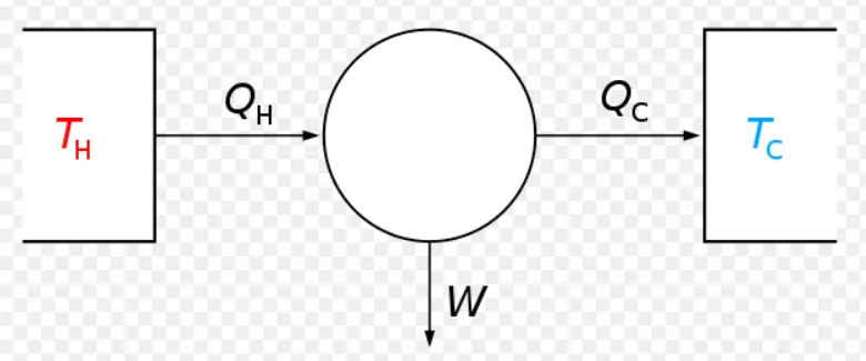
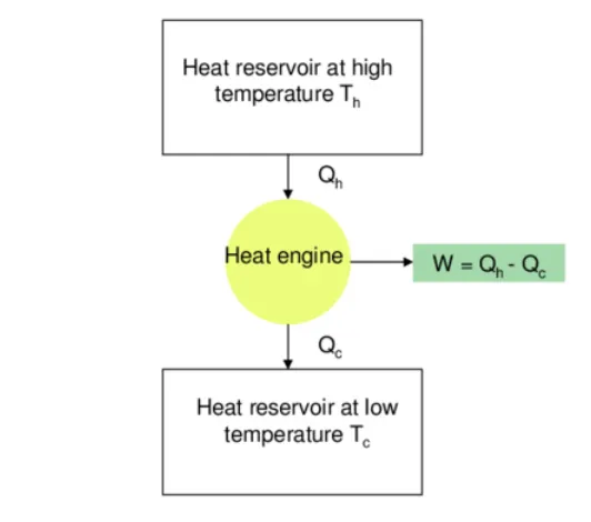
The high heat of working fluid vaporization places a restriction on the Rankine cycle's efficacy. The temperature range that the cycle can operate across is also fairly limited, with steam turbine entry temperatures normally being around 565 °C and steam condenser temperatures being around 30 °C, unless the pressure and temperature in the steam boiler reach super critical levels. In comparison to an actual overall thermal efficiency of up to 42% for a modern coal-fired power plant, this results in a theoretical maximum Carnot efficiency for the steam turbine alone of roughly 63.8%. The Rankine (steam) cycle is frequently employed as a bottoming cycle in combined-cycle gas turbines to recover heat that would otherwise be rejected due to the lower steam turbine entry temperature (relative to a gas turbine).

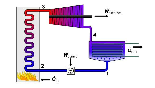
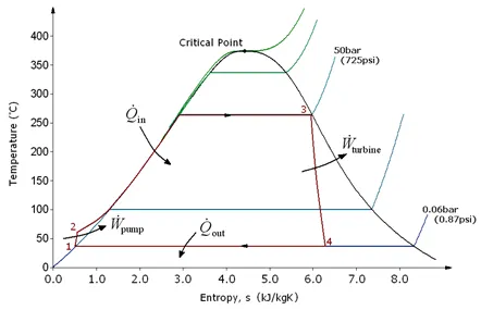
In these power plants, cooling towers and a huge body of water are typically used as the cold source—the colder, the better (river or sea). The lower practical temperature of the working fluid restricts the Rankine cycle's efficiency on the cold side. In a Rankine cycle, the working fluid follows a closed loop and is continuously recycled. The cooling systems are what produce the water vapor with condensed droplets that are frequently observed blowing from power plants (not directly from the closed-loop Rankine power cycle). The "Qout" streaming out of the lower side of the cycle in the T-s figure below represents this "exhaust" heat. In order to function as a huge heat exchanger, cooling towers must first absorb the latent heat of vaporization of the working fluid and simultaneously evaporating cooling water to the atmosphere.

Although a variety of materials could be used as the working fluid in the Rankine cycle, water is typically the fluid of choice because of its beneficial characteristics, including its abundance, low cost, and non-toxic and unreactive chemistry. It is also the fluid of choice because of its thermodynamic properties. The pressure at the turbine outlet is reduced by condensing the working steam vapor to a liquid, and the energy used by the feed pump uses just 1% to 3% of the turbine's output power, increasing the cycle's efficiency. The advantage of this is negated by the low steam temperature permitted to the turbine (s). Turbine entry temperatures for gas turbines, for instance, are close to 1500 °C. However, thermal efficiency of the actual huge steam power stations and large modern gas turbine stations are similar.

PROCESSES - RANKINE CYCLE:

The Rankine cycle is a thermodynamic cycle that describes the operation of a steam turbine. It consists of four main stages:

1. Process 1-2 : Isentropic compression - Heat addition at constant pressure in the boiler
2. Process 2-3 : Constant pressure heat addition in boiler - Expansion through the turbine
3. Process 3-4 : Isentropic expansion - Heat rejection at constant pressure in the condenser
4. Process 4-1 : Constant pressure heat rejection in condenser - Pumping of the working fluid to the boiler pressure

THERMODYNAMIC EQUATIONS:

Application of the First law of thermodynamics to the control volume (pump, steam generator, turbine and condenser), gives: [2]

Work done on pump, per kg of water:

Heat energy added in steam generator:

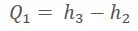
Work delivered by turbine:

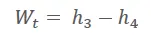
Heat energy rejected in the condenser:

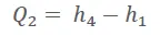
Net-Work done is given by:

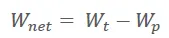
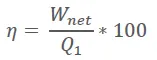
The thermal efficiency of the Rankine cycle is given by:

Also, the thermal efficiency can also be identified as:

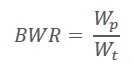
Back Work Ratio is given by:

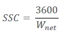
Specific Steam Consumption:

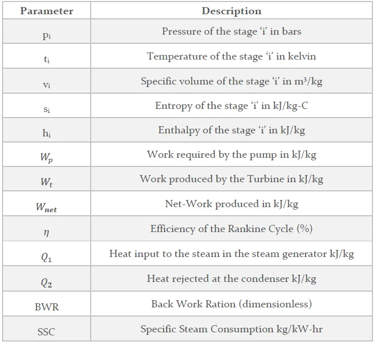
VARIABLE DETAILS:

The list of variables is used to define the thermodynamic equations of the Rankine Cycle are mentioned below:

MATLAB CODE:

%RANKINE CYCLE SIMULATOR
%CALCULATING THE NETWORK OF THE RANKINE CYCLE
%CALCULATING THE BACK WORK RATIO OF THE RANKINE CYCLE
%TAKING VALUES FROM THE USER
 
clear all
close all
clc
 
%DISPLAYING THE CONTENT 
fprintf("\n                                RANKINE CYCLE SIMULATOR            \n");
fprintf("\n Process 1-2 : Isentropic expansion in the Turbine \n");
fprintf("\n Process 2-3 : Isobaric heat rejection by the Condenser \n");
fprintf("\n Process 3-4 : Isentropic compression in the Pump \n");
fprintf("\n Process 4-1 : Isobaric heat addition by the Boiler \n");
 
%REQUESTING THE USER TO GIVE THE INPUTS
p1 = input('\n Enter the pressure at the Turbine inlet (in bar) = ');
t1 = input('\n Enter the temperature at the Turbine inlet (in Celsius) = ');
p2 = input('\n Enter the pressure at the Condenser (in bar) = ');
 
%TURBINE INLET PARAMETERS
tsat_1 = XSteam('Tsat_p',p1);
if t1 > tsat_1
    h1 = XSteam('h_pt',p1,t1);
    s1 = XSteam('s_pt',p1,t1);
elseif t1 == tsat_1
        h1 = XSteam('hV_p',p1);
        s1 = XSteam('sV_p',p1);
    else 
        fprintf("\n Enter higher value of Turbine inlet temperature (in Celsius)!!! \n\n");
end
 
 
%CONDITIONS AT TURBINE OUTLET
%BASED ON THE LOCATION OF POINT 2 THE FOLLOWING VALUES/PROPERTIES ARE
%EVALUATED
s2 = s1; %isentropic expansion in the turbine
ssat_2 = XSteam('sV_p',p2);
if s2 < ssat_2
    sf_2 = XSteam('sL_p',p2);
    sg_2 = XSteam('sV_p',p2);
    %let x denote the dryness fraction of the steam in the system
    x = (s2 - sf_2)/(sg_2 - sf_2);
    hf_2 = XSteam('hL_p',p2);
    hg_2 = XSteam('hV_p',p2);
    h2  = hf_2 + x*(hg_2 - hf_2);
    t2 = XSteam('Tsat_p',p2);
else
    x = 1;
    h2 = XSteam('hV_p',p2);
    t2 = XSteam('Tsat_p',p2);
end
 
 
%CONDITIONS AT PUMP INLET
p3 = p2;
t3 = XSteam('Tsat_p',p3);
h3 = XSteam('hL_p',p3);
s3 = XSteam('sL_p',p3);
v3 = XSteam('vL_p',p3);
 
 
%CONDITIONS AT BOILER INLET
p4 = p1;
s4 = s3; 
v4 = XSteam('v_ps',p4,s4);
cp4 = XSteam('Cp_ps',p4,s4);
cv4 = XSteam('Cv_ps',p4,s4);
gamma = cp4/cv4;
G = (gamma - 1)/gamma;
t4 = t3*(p2/p1)^G;
 
%WORK REQUIRED BY THE PUMP
W_p = v3*(p4 - p3)*100;
%W_p = h4 - h3
h4 = W_p + h3;
 
 
 
%CONDITION OF INTERMEDIATE STATES: STATE 5 AND STATE 6 IN (4-1) STAGE
t5 = XSteam('Tsat_p',p4);
s5 = XSteam('sL_p',p4);
t6 = t5;
s6 = XSteam('sV_p',p4);
 
 
%WORK DONE BY THE TURBINE
W_t = h1 - h2;
 
%HEAT INPUT
Q_in = h1 - h4;
 
%HEAT OUTPUT
Q_out = h2 - h3;
 
%NET-WORK OBTAINED
W_net = W_t - W_p;
 
%Efficiency of the Rankine Cycle
efficiency = (W_net*100)/Q_in;
 
%BACK WORK RATIO
BWR = W_p/W_t;
 
%SPECIFIC STEAM COSUMPTION
SSC = 3600/W_net;
 
 
%DISPLAYING THE OBTAINED INFORMATION
fprintf("\n                                RESULTS            \n");
fprintf("At State Point 1:                              At State Point 4: \n P1 = %.2f bar                                 P4 = %.2f bar \n T1 = %.2f C                                  T4 = %.2f C  \n H1 = %.2f kJ/kg                             H4 = %.2f kJ/kg  \n S1 = %.2f kJ/kg-C                              S4 = %.2f kJ/kg-C \n",p1,p4,t1,t4,h1,h4,s1,s4);
fprintf("\nAt State Point 2:                              At State Point 3: \n P2 = %.2f bar                                  P3 = %.2f bar \n T2 = %.2f C                                   T3 = %.2f C  \n H2 = %.2f kJ/kg                             H3 = %.2f kJ/kg  \n S2 = %.2f kJ/kg-C                              S3 = %.2f kJ/kg-C \n",p2,p3,t2,t3,h2,h3,s2,s3);
 
fprintf("\n Work required by the pump in the Rankine Cycle = %.2f kJ/kg\n",W_p);
fprintf("\n Work produced by the turbine in the Rankine Cycle = %.2f kJ/kg\n",W_t);
fprintf("\n Net Work obtained in the Rankine Cycle = %.2f kJ/kg\n",W_net);
fprintf("\n Heat input to the Rankine Cycle = %.2f kJ/kg\n",Q_in);
fprintf("\n The efficiency of the Rankine Cycle = %.2f \n",efficiency);
fprintf("\n Back Work Ratio in the Rankine Cycle = %.9f \n",BWR);
fprintf("\n Specific Steam Consumption in the Rankine Cycle = %.2f kg/kWh \n",SSC);
 
 
%PLOTTING THE CURVES
 
%Plotting Rankine Cycle TS DIAGRAM
%Plotting Saturation Curve
T = linspace(0,373.946,100); % critical point of water occurs at 373.946 degreeC
figure(1);
hold on
for i = 1 : length(T)
    s_l(i) = XSteam('sL_T',T(i));
    s_g(i) = XSteam('sV_T',T(i));
    h_l(i) = XSteam('hL_T',T(i));
    h_g(i) = XSteam('hV_T',T(i));
end
 
plot(s_l,T,'linewidth',3,'color','g');
plot(s_g,T,'linewidth',3,'color','g');
plot([s1 s2],[t1 t2],'linewidth',1,'color','k');
text(s1,t1,'1'); 
plot([s2 s3],[t2 t3],'linewidth',1,'color','r');
text(s2,t2,'2');
plot([s3 s4],[t3 t4],'linewidth',1,'color','k');
text(s3,t3,'3');
plot([s4 s5],[t4 t5],'linewidth',1,'color','r');
text(s4,t4,'4');
plot([s5 s6],[t5 t6],'linewidth',1,'color','r');
text(s5,t5,'5');
plot([s6 s1],[t6 t1],'linewidth',1,'color','r');
text(s6,t6,'6');
xlabel('Entropy (kJ/kg-C)');
ylabel('Temperature (C)');
title('Entropy versus Temperature Curve - Rankine Cycle');
legend('Entropy (s)kJ/kg-C','Temperature (t)C');
grid on
hold off
 
 
%Plotting Rankine Cycle HS DIAGRAM
%Plotting Saturation Curve
figure(2);
hold on
plot(s_l,h_l,'linewidth',3,'color','c');
plot(s_g,h_g,'linewidth',3,'color','c');
plot([s1 s2],[h1 h2],'linewidth',1,'color','k');
text(s1,h1,'1');
plot([s2 s3],[h2 h3],'linewidth',1,'color','r');
text(s2,h2,'2');
plot([s3 s4],[h3 h4],'linewidth',1,'color','k');
text(s3,h3,'3');
plot([s4 s1],[h4 h1],'linewidth',1,'color','r');
text(s4,h4,'4');
xlabel('Entropy (kJ/kg-C)');
ylabel('Enthalpy (kJ/kg)');
title('Enthalpy versus Entropy Curve - Rankine Cycle');
legend('Entropy (s)kJ/kg-C','Enthalpy (h)kJ/kg');
grid on
hold off

CODE EXPLANATION:

The Rankine Cycle is introduced to the user at the outset of the code, along with information on the process and its nature.
The user is then given comments to input into the data. which accepts p2, t1, and p1 parameters.

The specifications for the turbine inlet are set. Initially, a MATLAb specified function called XSteam is used to determine the saturation temperature at pressure p1.
At pressure p1 and temperature t1, the values of h1 and s1 are invoked using XSteam if the turbine inlet temperature is higher than the saturation temperature.

The enthalpy and entropy occur in the vapour area if the temperature t1 is equal to the saturation temperature, and XSteam can invoke the values of these quantities at the pressure p1.
The if and else-if conditions are used to calculate these numbers.
A different value of turbine inlet temperature is needed to conduct the Rankine Cycle if the temperature does not meet either of these requirements.
It is clear from the procedure that stage 1 to stage 2 in the turbine where work is created includes isentropic expansion, i.e., s2 = s1.
If the entropy at state 2 is lower than the saturated entropy value at pressure p2 (i.e., s2 ssat2), then dryness percentage must be taken into account.

XSteam is used to determine the entropy of saturated liquid and saturated vapour at pressure p2.
The following formula is used to compute dryness fraction value:

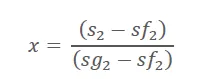
The dryness fraction and the enthalpy values received from the XSteam function at pressure p2 are used to compute the value of the enthalpy at state 2.
At pressure p2, the temperature t2 corresponds to the saturation temperature.
The dryness fraction is 1 in all other cases. The values of enthalpy and temperature are then given, with h2 standing for the enthalpy of a saturated liquid at pressure p2 and t2 for the saturated temperature at p2.
The if and else statements are used to calculate the values listed above.

According to the Rankine cycle hypothesis, stage 2 to stage 3 involve isobaric heat rejection, hence p3 = p2.
A fairly simple method of calculating the pump inlet conditions involves calling the XSteam function directly at pressure p3. Calculated quantities include temperature (saturation), specific volume, enthalpy, and entropy.
Isentropic compression, which happens in the pump, is process 3–4. In this, states 3 and 4 have equal entropies, or s4 = s3.
The steam generator's process 4-1 is an isobar heat addition process, therefore the pressures in states 1 and 4 are equal, or p4 = p1.

Utilizing the XSteam function, the specific volume at stage 4 is determined with values to be calculated at pressure p4 and entropy s4. Using the XSteam function, the values of specific heat at constant pressure and volume at state 4 are calculated using the same pressure and entropy parameters.
The ratio of specific heat at constant pressure to that at constant volume is used to determine the adiabatic index.
The temperature of the state 4 is determined using the adiabatic gas law.
The variables v3, p4, and p3 are used to compute the work performed by the pump.

As noted in the section on thermodynamic relations, the value of enthalpy at state 4 is determined using the work performed by the pump and the known value of h3.
The temperature of the process 4-1 intersects the saturated liquid line on the TS curve at state 5, where state 5's entropy is equal to the entropy of the saturated liquid at state 4, and the temperature corresponds to the saturated temperature at p4.
The saturated vapour line is reached by the same method (4-1) at point 6, where the temperature is the same as it was at point 5 (t6 = t5). Additionally, the entropy at point 6 matches that of the saturated vapour at point 4 (p4).

As discussed in the previous section, the values of work done by the turbine, heat input, heat rejected, net work, efficiency, back work ratio, and specific steam consumption are computed.
A numerical array T is given to draw the saturation curve in the TS diagram, and using linspace, the values are ranged from 0°C to 373.946°C (the water's critical point), with the range being divided into 100 equal parts.
The values of entropy and enthalpy at the saturated liquid and saturated vapour phases are used to calculate the saturated values that will be depicted on figure (1). A for loop is run along the length of the numerical temperature array T to calculate these values.

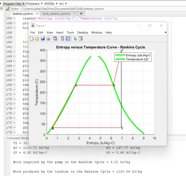
While plotting the saturation curve on TS curve, the values of entropy from the for loop are quoted along with the temperature array separately for saturated liquid and saturated vapour. The linewidth is maintained at 3 and is coloured in green.

The other points are plotted as mentioned below:

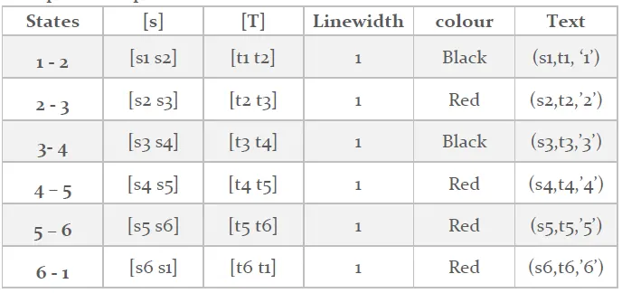
A legend is written along with labelling the axes. The plot is titled as “Temperature versus Entropy Curve - Rankine Cycle.”

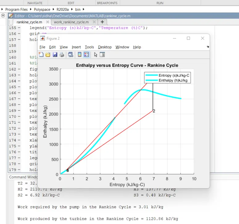
Similarly, the HS curve is plotted. While plotting the saturation curve on HS curve, the values of enthalpy from the for loop are quoted along with the temperature array separately for saturated liquid and saturated vapour. The linewidth is maintained at 3 and is coloured in cyan.

The other points are plotted as mentioned below:

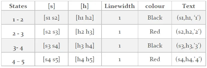
The axes are labeled and have a legend written alongside them. "Enthalpy against Entropy Curve - Rankine Cycle" is the plot's title.
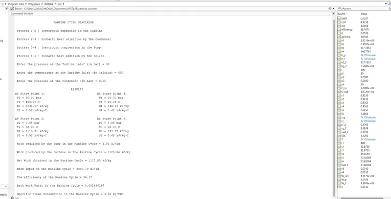
For each state, the values for pressure, temperature, enthalpy, and entropy are computed and printed in the command window along with the thermodynamic attributes.

OUTPUT:

COMMAND WINDOW:

RESULT:

PLOT 1: ENTROPY VS TEMPERATURE CURVE

PLOT 2: ENTHALPY VS ENTROPY CURVE

CONCLUSION:

The code follows the theoretically ideal Rankine cycle exactly and is quite simple.
Utilizing the XSteam function with the proper input parameters, such as pressure and temperature, is very crucial. The Rankine Cycle theory must be thoroughly understood to accomplish this.

The TS and HS plots of the Rankine cycle according to the problem statement have been plotted by from an appropriate code written in MATLAB as shown in the figures below. The thermal efficiency of the Rankine cycle is evaluated and was found to be 36.17 % and the back work ratio was found to be 0.00268.