Project 2 - Rankine cycle Simulator
Title : Rankine cycle Simulator using MATLAB
Objectives :
- Create a Rankine Cycle Simulator using MATLAB
- To calculate the state points of the Rankine Cycle
- Plot the corresponding T-s and h-s plots for the given set of inputs and also give suitable title and label for the same
Introduction
A Rankine cycle power system is a heat engine converting thermal energy into work. The Rankine cycle is named after William John Macquorn Rankine, a Scottish polymath professor at Glasgow University. Similar to the vapor compression heat pump, it comprises four main components: a boiler (sometimes called evaporator), a turbine, a condenser and a pump. The working fluid in a low-pressure slightly subcooled liquid state is brought to high pressure by the pump. The pump consumes power. The high-pressure liquid enters the boiler, where it is heated-up, vaporized and potentially heated again to leave the boiler in superheated vapor state. At the outlet of the boiler, the high-pressure vapor enters the turbine where it is expanded down to the low pressure. The turbine delivers mechanical power. At the outlet of the turbine, the fluid enters the condenser where it is condensed to liquid state and, then, slightly subcooled. Thermal power rejected at the condenser is dumped into a heat sink. The low-pressure subcooled liquid enters the pump again. The net power delivered by the Rankine cycle system is the power delivered by the turbine minus that consumed by the pump. [1]
The Rankine cycle power system is the technology employed in steam power plants for the electricity production. These conventional steam Rankine cycle power systems use water as the working fluid. Other working fluids than water can be used.
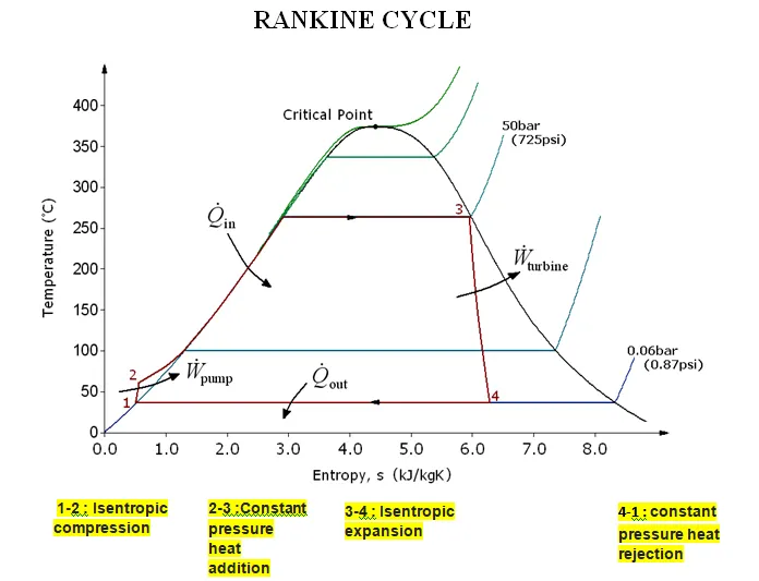
Processes of Rankine Cycle
- Process 1–2: Process 1-2 is isentropic compression. The working fluid is pumped from low to high pressure. As the fluid is a liquid at this stage, the pump requires little input energy. The working fluid is pushed from low to high pressure in this chamber.
- Process 2–3: Process 2-3 is constant pressure heat addition in boiler. The high-pressure liquid is introduced to the boiler and cooked at constant pressure to become a dry saturated vapour in this process.
- Process 3-4: Isentropic expansion in a turbine. Power is generated as the dry saturated vapour expands through the turbine.
- Process 4-1: Heat rejection under constant pressure in a condenser. A saturated liquid is formed by condensing wet vapour at a steady pressure.
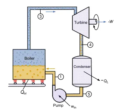
In an ideal Rankine cycle the pump and turbine would be isentropic, i.e., the pump and turbine would generate no entropy and hence maximize the net work output.
Variables used to calculate the efficiency for Rankine cycle
Temperature : Temperature is a thermal state of a body which distinguishes a hot body from a cold body. Unit of temperature Celcius.
Pressure : Pressure is the force applied perpendicular to the surface of an object per unit area. Pressure = Force/Area. Unit of pressure is N/m^2. 1 bar = 10^5 N/m^2.
Entropy : In a simple words, entropy is the measure of a system's thermal energy per unit temperature that is unavailable for doing useful work. It is donated as S and unit is J/K.mol.
Enthalpy : Enthalpy, a property of a thermodynamic system, is the sum of the system's internal energy and the product of its pressure and volume. It is denoted as H . Enthalpy (H) = Internal energy (E) + PV . Unit of enthalpy is Joule .
MATLAB SCRIPT FILE
clear all    %Clear all existing  variables from workspace
close all    %Close the figure windows
clc          %Clear the command window

%% Printing the title of the project and the processess involved
fprintf('------------------------------------------- RANKINE CYCLE SIMULATOR -----------------------------------------------------------------\n');

%Printing all the four process in Rankine Cycle
fprintf('Process 1-2 is Isentropic Expansion in the Turbine\n')
fprintf('Process 2-3 is Constant Pressure Heat Rejection by the Condenser\n')
fprintf('Process 3-4 is Isentropic Compression in the Pump\n')
fprintf('Process 4-1 is Constant Pressure Heat Addition by the Boiler\n')

%% Inputs
%Pressure (P1) at Turbine Inlet
P1 = input('Enter the Pressure at Turbine Inlet = ');

%Temperature (T1) at Turbine Inlet
T1 = input('Enter the Temperature at Turbine Inlet = ');

%Pressure (P3) at Condenser Inet
P2 = input('Enter the Pressure at Turbine Outlet = ');

%%
% CALCULATING THE THERMODYNAMIC PROPERTIES IN ALL FOUR STATE POINTS
% AT STATE POINT 1
%Enthalpy (H1)
H1 = XSteam('h_pt',P1,T1);

%Entropy (S1)
S1 = XSteam('s_pt',P1,T1);

%% AT STATE POINT 2
%Entropy (S2)
% Isentropic process (Entropy = constant)
S2 = S1;

% Calculating X2
sf2 = XSteam('sL_p',P2);
sg2 = XSteam('sV_p',P2);
hf2 = XSteam('hL_p',P2);
hg2 = XSteam('hV_p',P2);
X2 = ((S2-sf2)/(sg2-sf2));

% Enthalpy (H2)
H2 = (hf2 + (X2*(hg2-hf2)));

% Temperature (T2)
T2 = XSteam('T_ps',P2,S2);

%% AT STATE POINT 3

%Pressure (P3)
%Constant Pressure Heat Addition
P3 = P2;

%Temperature is constant in condenser
T3 = T2;

% Enthalpy (H3)
H3 = XSteam('hL_p',P3);

% Entropy (S3)
S3 = XSteam('sL_p',P3);

%% STATE POINT 4
% Entropy (S4)
% Isentropic process(Entropy = constant)
S4 = S3;

% Pressure (P4)
% Constant Pressure Heat Rejection
P4 = P1;

% Enthalpy (H4)
H4 = XSteam('h_ps',P4,S4);

% Temperature (T4)
T4 = XSteam('T_hs',H4,S4);

% STATE POINT 5
% Temperature (T5)
T5 = XSteam('Tsat_p',P4);

% Entropy (S5)
S5 = XSteam('sL_p',P4);

% STATE POINT 6
% Temperature (T6)
T6 = T5;

% Entropy (S6)
S6 = XSteam('sV_T',T6);

% Rankine Cycle Parameters
% Turbine Work
Wt = H1-H2;

% Pump Work
Wp = H4-H3;

% Net Work Done
Wnet = Wt - Wp;

% Heat Supplied
Qin = H1-H4;

% Heat Rejected
Qout = H2-H3;

% Efficiency of Rankine Cycle
Eff = (Wnet/Qin)*100;

% Back Work Ratio
BWR = (Wp/Wt);

% Specific Steam Consumption
SSC = 3600/Wt;

%% Printing the evaluated parameters
fprintf('------------------------------------------- RESULTS -----------------------------------------------------------------\n');

% State Point 1
fprintf('At State Point 1:\n');
fprintf('Enthalpy (H1) is : %0.2f KJ/Kg\n',H1);
fprintf('Entropy (S1) is : %0.2f KJ/Kgk\n',S1);
fprintf('Temperature (T1) is : %0.2f Degree Celcius\n',T1);
fprintf('Pressure (P1) is : %0.2f Bar\n',P1);

% State Point 2
fprintf('At State Point 2\n');
fprintf('Enthalpy (H2) is : %0.2f KJ/Kg\n',H2);
fprintf('Entropy (S2) is : %0.2f KJ/Kgk\n',S2);
fprintf('Temperature (T2) is : %0.2f Degree Celcius\n',T2);
fprintf('Pressure (P2) is : %0.2f Bar\n',P2);

% State Point 3
fprintf('At State Point 3,\n');
fprintf('Enthalpy (H3) is : %0.2f KJ/Kg\n',H3);
fprintf('Entropy (S3) is : %0.2f KJ/Kgk\n',S3);
fprintf('Temperature (T3) is : %0.2f Degree Celcius\n',T3);
fprintf('Pressure (P3) is : %0.2f Bar\n',P3);

% State Point 4
fprintf('At State Point 4\n');
fprintf('Enthalpy (H4) is : %0.2f KJ/Kg\n',H4);
fprintf('Entropy (S4) is : %0.2f KJ/Kgk\n',S4);
fprintf('Temperature (T4) is : %0.2f Degree Celcius\n',T4);
fprintf('Pressure (P4) is : %0.2f Bar\n',P4);
fprintf('------------------------------------------- RANKINE CYCLE PARAMETERS -----------------------------------------------------------------\n');

% Turbine Work
fprintf('Work Done by the Turbine is : %0.2f KJ/Kg\n',Wt);
fprintf('Work Done by the Pump is : %0.2f KJ/Kg\n',Wp);
fprintf('Net Work Done is : %0.2f KJ/Kg\n',Wnet);
fprintf('Efficiency of the Rankine Cycle is : %0.2f Percantage\n',Eff);
fprintf('Back Work Ratio of the Cycle is : %f \n',BWR);
fprintf('S.S.C of the Cycle is : %0.2f Kg/KWh\n',SSC);

%% Plotting the graphs

% HS Diagram
% Points for Saturation Curve
s_c = (1:1000);
for i = 1:1000
    s_l(i) = XSteam('sL_T',i);
    h_l(i) = XSteam('hL_T',i);
    s_v(i) = XSteam('sV_T',i);
    h_v(i) = XSteam('hV_T',i);
end

%Saturation Curuve
figure(1)
plot(s_l,h_l,'-','linewidth',1.5,'color','r')
hold on
plot(s_v,h_v,'-','linewidth',1.5,'color','r')

% State Points
plot([S1 S2 S3 S4 S1],[H1 H2 H3 H4 H1],'linewidth',2,'color','blue')
text(S1,H1,'1')
text(S2,H2,'2')
text(S3,H3-50,'3')
text(S4,H4+100,'4')
xlabel('Entropy (KJ/Kg-K)')
ylabel('Enthalpy (KJ/Kg)')
title('H-S Diagram')
grid on
hold off

%TS Diagram
% Saturation Curve
figure(2)

plot(s_l,s_c,'-','linewidth',1.5,'color','r')
hold on
plot(s_v,s_c,'-','linewidth',1.5,'color','r')

% State Points
plot([S1 S2 S3 S4 S5 S6 S1],[T1 T2 T3 T4 T5 T6 T1],'linewidth',2,'color','blue')
xlabel('Entropy (KJ/Kg-K)')
text(S1,T1,'1')
text(S2,T2,'2')
text(S3,T3-15,'3')
text(S4,T4+20,'4')
ylabel('Temperature (Degree Celcius)')
title('T-S Diagram')
grid on
Explanation of the code :
- First of all as usual in order to clear the previous existing variables in workspace , to close the figure windows and to clear the command window clear all, close all and cls has been used.
- Then, we have printed the name of the processes according to the order and assigned the inputs for this case such as Turbina inlet and outlet pressure and temperature at inlet of the turbine.
- After that, calculation has been done for all of the four state points by calling function according to the requirements from the given Xsteam table file in question statements such as Entropy, Enthalpy, Temperature,Pressure, etc..
- Next we have evaluated the Rankine cycle parameters like turbina work, back ratio, efficiency,etc.. using the standard formula for rankine cycle.
- Then, as we wanted to get the values of the variables in command window, so using the MATLAB in-built command 'fprintf' we print all the variables for all the four state in command window.
- From the next line, plotting has been done of in twi different figure windows using 'figure' command.
- Also, we have added more suitable axis , label and to visualize the processes clearly in the graph 'text' command has used.
- In this way, we have written down our MATLAB code for the Rankine cycle simulator.
Outputs :
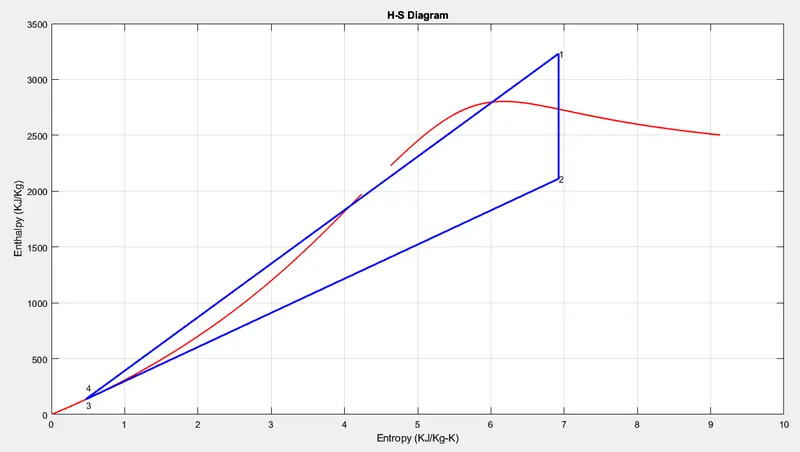
Enthalpy Vs Entropy diagram
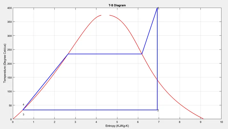
Temperature Vs Entropy diagram
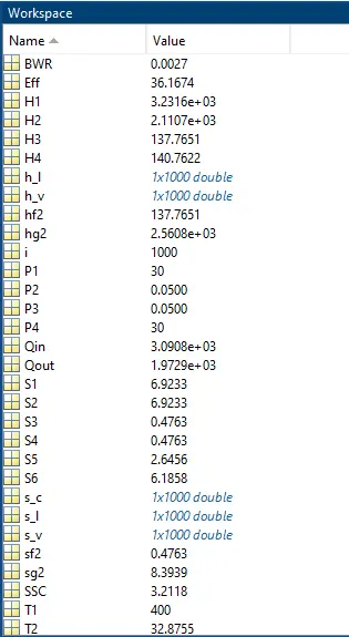
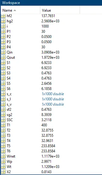
Screenshots of Workspace variables
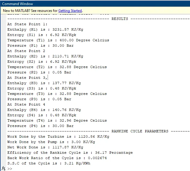
Screenshots of command window
------------------------------------------- RANKINE CYCLE SIMULATOR -----------------------------------------------------------------
Process 1-2 is Isentropic Expansion in the Turbine
Process 2-3 is Constant Pressure Heat Rejection by the Condenser
Process 3-4 is Isentropic Compression in the Pump
Process 4-1 is Constant Pressure Heat Addition by the Boiler
Enter the Pressure at Turbine Inlet = 30
Enter the Temperature at Turbine Inlet = 400
Enter the Pressure at Turbine Outlet = 0.05
------------------------------------------- RESULTS -----------------------------------------------------------------
At State Point 1:
Enthalpy (H1) is : 3231.57 KJ/Kg
Entropy (S1) is : 6.92 KJ/Kgk
Temperature (T1) is : 400.00 Degree Celcius
Pressure (P1) is : 30.00 Bar
At State Point 2
Enthalpy (H2) is : 2110.71 KJ/Kg
Entropy (S2) is : 6.92 KJ/Kgk
Temperature (T2) is : 32.88 Degree Celcius
Pressure (P2) is : 0.05 Bar
At State Point 3,
Enthalpy (H3) is : 137.77 KJ/Kg
Entropy (S3) is : 0.48 KJ/Kgk
Temperature (T3) is : 32.88 Degree Celcius
Pressure (P3) is : 0.05 Bar
At State Point 4
Enthalpy (H4) is : 140.76 KJ/Kg
Entropy (S4) is : 0.48 KJ/Kgk
Temperature (T4) is : 32.96 Degree Celcius
Pressure (P4) is : 30.00 Bar
------------------------------------------- RANKINE CYCLE PARAMETERS -----------------------------------------------------------------
Work Done by the Turbine is : 1120.86 KJ/Kg
Work Done by the Pump is : 3.00 KJ/Kg
Net Work Done is : 1117.87 KJ/Kg
Efficiency of the Rankine Cycle is : 36.17 Percantage
Back Work Ratio of the Cycle is : 0.002674
S.S.C of the Cycle is : 3.21 Kg/KWh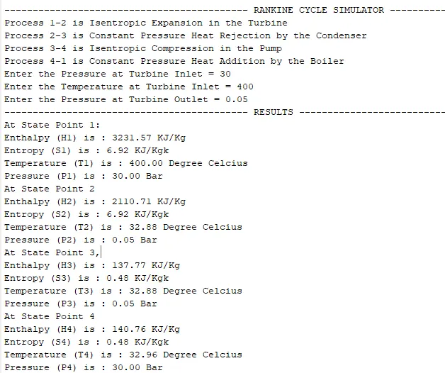
Conclusion :
- We have understood the working process of Rankine cycle and also the processes involves in Rankine cycle .
- We have calculated the variables at four stste points using the given Xsteam library and also created the Rankine cycle simulator using MATLAB.
- Plotting has been done for the Enthalpy Vs Entropy and Temperature vs Entropy.
- So,at the end we have successfully completed the project of Rankine cycle simulator.
References :
1. https://www.sciencedirect.com/topics/earth-and-planetary-sciences/rankine-cycle