Project 2 - Rankine cycle Simulator

AIM :-

     To Understand the concept of Rankine cycle by referring to standard thermal engineering text book.

• Create a Rankine Cycle Simulator using OCTAVE/MATLAB.
• Your code should calculate the state points of the Rankine Cycle (any type of your choice) based on user inputs. 
• Then, plot the corresponding T-s and h-s plots for the given set of inputs. Title and axes labels are a must, while legends could be used if necessary.

OBJECTIVE :- 

     Obtain the plots of T-s and h-s.  

THEROY:-

      Rankine cycle 

      The Rankine cycle is an idealized thermodynamics cycle descriribing the process by which certainheat engines, such as steam turbines or reciprocating steam engines,            allow mechanical work to be extracted from a fluid as it moves between a heat source and heat sink.

    Rankine cycle model:

       process 

        1 - 2  isentropic expansion in turbine

        2 - 3  constant pressure heat Rejection by condenser

        3 - 4  isentropic compression in pump

        4 - 1  constant pressure Heat addition by boiler.

    MATLAB CODING   

clear all
close all
clc
p1 = input('Enter a Value of pressure at turbine inlet, p1 = ');
p2 = input('Enter a Value of pressure at condenser inlet, p2 = ');
T1 = input('Enter a Value of temperature at turbine inlet, T1 = ');

 
% State 1
 h1 = XSteam('h_pT', p1, T1);          % Extracting Enthalpy at state pt 1
 s1 = XSteam('s_pT', p1, T1);  

% At State 2
  s2 = s1;                              % Isentropic Expansion                
  sf2= XSteam('sL_p', p2);              % Saturated Liquid Entropy
  sg2 = XSteam('sV_p', p2);             % Saturated Vapour Entropy
  x2 = (s2-sf2)/(sg2-sf2);
  hf2 = XSteam('hL_p', p2);           
  hg2 = XSteam('hV_p', p2);
  h2 = hf2 + (x2*(hg2-hf2));

% At State 3
  p3 = p2;                              % Constant pressure Heat rejection in Condenser
  s3= XSteam('sL_p', p3);
  h3 = XSteam('hL_p', p3);

% At State 4
  s4 = s3;
  p4 = p1;


Wt = h1 - h2;                             % Work done by turbine

v3 = XSteam('vL_p', p3);                  % Work done to run pump
Wp = v3*(p4 - p3)*100;
h4 = h3 + Wp;

Wnet = Wt - Wp;                           % Net work

Qin = h1 - h4;                            % Heat into the system

Qout = h2 - h3;                           % Heat out of the system

thermal_eff = (Wnet/Qin)*100;             % Thermal efficiency

SSC = (3600/Wnet);                        % Specific Steam Consumption

BW = (Wp/Wt);                             % Back Work ratio


% Calculation of Temperatures at the state points
  T3 = XSteam('Tsat_p', p3);
  T2 = T3;
  Cp4 = XSteam('Cp_ps', p4, s4);
  Cv4 = XSteam('Cv_ps', p4, s4);
  k = Cp4/Cv4;
  T4 = T3/((p3/p4)^((k-1)/k));



% Calculating Temperature, Entropy and Enthalpy at the vapour and liquid line for plotting
 T6 = XSteam('Tsat_p', p1);
 s5 = XSteam('sL_p', p1);
 s6 = XSteam('sV_p', p1);
 h5 = XSteam('hL_p', p1);
 h6 = XSteam('hV_p', p1);
 T5 = T6;


% Plotting the saturation curve
  T = linspace(1,375,1000);
  for i = 1:length(T)
     sf(i) = XSteam('sL_T', T(i));
     sg(i) = XSteam('sV_T', T(i));
     hf(i) = XSteam('hL_T', T(i));
     hg(i) = XSteam('hV_T', T(i));

  end


% Plotting T-s diagram
  figure(1)
  hold on
  plot(sf, T, 'r','linewidth',1)
  plot(sg, T, 'r','linewidth',1)
  plot([s1 s2], [T1 T2], 'b', 'linewidth', 2)
  plot([s2 s3], [T2 T3] ,'b', 'linewidth', 2)
  plot([s3 s4], [T3 T4], 'b', 'linewidth', 2)
  plot([s4 s5], [T4 T5], 'b', 'linewidth', 2)
  plot([s5 s6], [T5 T6], 'b', 'linewidth', 2)
  sc1 = linspace(s6, s1, 1000);
  for l = 1:length(sc1)
    Tc1(l) = XSteam('T_ps', p1, sc1(l));
  end
  plot(sc1, Tc1, 'b', 'linewidth', 2)
  title('Temp vs Entropy plot')
  xlabel('Entropy ,S (Kj/kgk')
  ylabel('Temperature (degree C) ')
  legend('Saturation curve')


% Plotting h-s diagram
  figure(2)
  hold on
  plot(sf, hf, 'k', 'linewidth', 1)
  plot(sg, hg, 'k',  'linewidth', 1)
  plot([s1 s2], [h1 h2], 'r', 'linewidth', 2)
  plot([s2 s3], [h2 h3], 'r', 'linewidth', 2)
  plot([s3 s4], [h3 h4], 'r', 'linewidth', 2)
  hc = linspace(h4, h5, 100);
  for r = 1:length(hc)
    sch(r) = XSteam('s_ph', p1, hc(r));
  end
  plot(sch,hc, 'r', 'linewidth', 2)
  plot([s5 s6], [h5 h6], 'r', 'linewidth', 2)
  for m = 1:length(sc1)
    hc1(m) = XSteam('h_ps', p1, sc1(m));
  end
  plot(sc1, hc1, 'r', 'linewidth', 2)
  title('Enthalpy vs Entropy plot')
  xlabel('Entropy , S (KJ/kgk) ')
  ylabel('Enthalpy , H (KJ/kg)')
  legend('Saturation curve','location','northwest')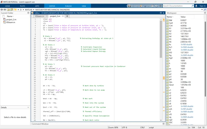

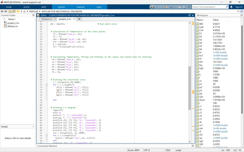
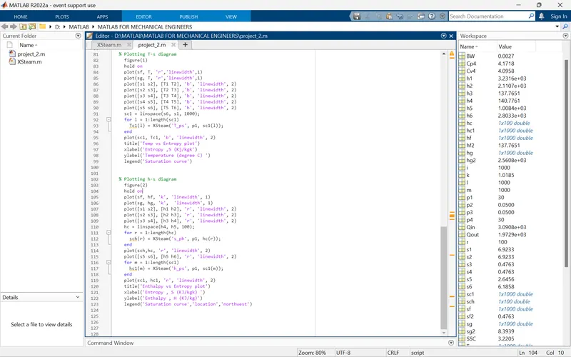
The cycle is coded to get input from the user. The input are inlet tempreature T1, inlet pressure P1 and  outlet pressure P2.

RESULTS :-   

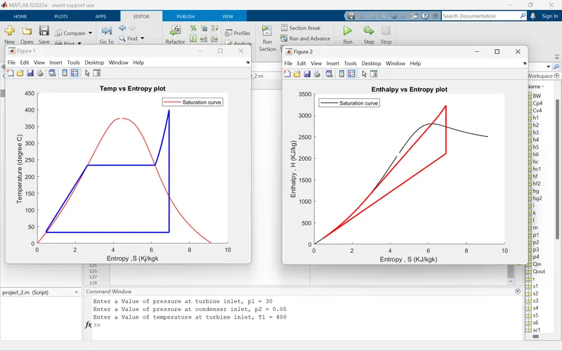
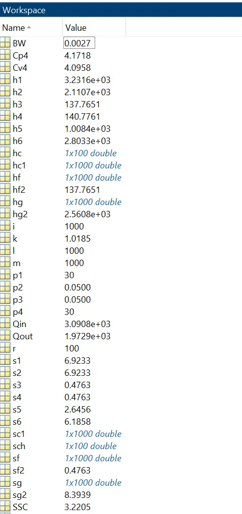
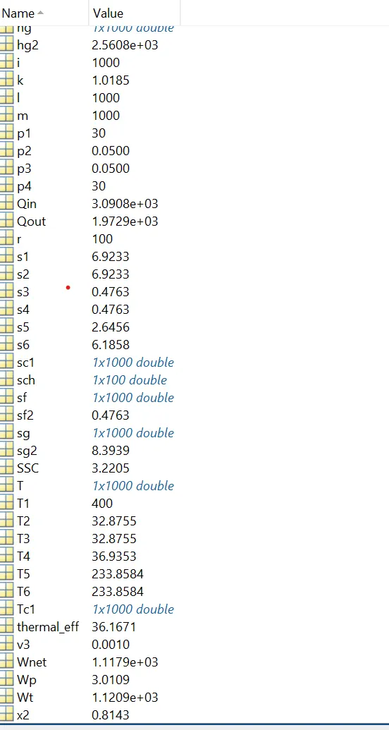
Here the plots of T - S  and  H - S  the cycle is run successfully and the results are updated in workspace.

Hence the Rankine cycle performance is observed with input parameters

The work space variables are given